Mohr's circle of tension

Mohr's circle of tension and construction

Figure 1: Mohr's circle for 2D stress state ${\displaystyle {\begin{bmatrix}\sigma _{xx}&\tau _{xy}\\\tau _{xy}&\sigma _{yy}\end{bmatrix}}={\begin{bmatrix}-1&4\\4&5\end{bmatrix}}}$

The Mohrsche Kreis or Mohrsche Stresskreis, named after Christian Otto Mohr , is a possibility to illustrate or examine the 3D stress state of a point or a volume of constant stress .

For this purpose, a free cut is made on an infinitesimal volume, whereby the traction vector t becomes visible on the cut surface. This traction vector, also known as the stress vector, is broken down into its component (also referred to here ) perpendicular to the interface (the so-called normal stress component) and its component (also referred to here ) parallel to the interface (the so-called shear stress component ). Depending on the angle at which the cut is made, pairs can be calculated and drawn as points in a diagram. The set of all points is Mohr's circle. At him z. B. read the principal stresses, the principal stress directions or the greatest shear stress. This gives you a clear idea of ​​the volume used. In the case of strength criteria such as failure criteria , flow criteria or elasticity limits of isotropic , homogeneous materials, only the principal stresses are relevant. For some strength criteria, only the stress in the plane of the greatest and smallest principal stress is relevant. Even in the computer age, the Mohr's circle of voltages is often used to assess them, because it quickly provides a clear solution. ${\displaystyle \sigma _{n}}$ ${\displaystyle t_{\bar {x}}}$ ${\displaystyle \tau _{n}}$ ${\displaystyle t_{\bar {y}}}$ ${\displaystyle \varphi }$ ${\displaystyle (t_{\bar {x}},t_{\bar {y}})}$

Mohr's circle can also be used to calculate the traction vector on any surface normal and thus the components of the stress tensor can be determined back: If the stress tensor components are given in relation to a Cartesian coordinate system, then the stress tensor components can be related with the Mohr's circle determine graphically on a Cartesian coordinate system. The prerequisite here is that the coordinate system emerges from the coordinate system through a rotation by the angle . ${\displaystyle (x,y)}$ ${\displaystyle ({\bar {x}},{\bar {y}})}$ ${\displaystyle ({\bar {x}},{\bar {y}})}$ ${\displaystyle \varphi }$ ${\displaystyle (x,y)}$

In addition to the Cauchy stress tensor, other symmetrical tensors can also be illustrated or investigated with Mohr's circle, e.g. B. the strain tensor . And besides Mohr's circle there are also other methods for illustrating symmetric tensors, e.g. B. Super squares or ellipsoids .

Mohr introduced the tension circle in 1882.

Cutting stress vector

(x, y) components

Figure 2: Particles with stress cut perpendicular to x (left) and at an angle (right), normal unit vector n, intersection stress vector t. ${\displaystyle \sigma }$ ${\displaystyle \varphi }$

The state of stress on a particle is determined by the symmetrical Cauchy stress tensor , which is usually defined as a (2.0) tensor. A cutout can be made in any direction on this particle and through its immediate surroundings. The cutting stress vector t (traction vector) can be calculated on the resulting cut surface . The relationship between the stress tensor and the intersection stress vector t is ${\displaystyle \sigma }$

${\displaystyle {\begin{aligned}t=\sigma \cdot n\end{aligned}},}$

where n is a normal unit vector that is perpendicular to the intersection and points “outwards”. The components of the voltage vector t with respect to the Cartesian - coordinate system are calculated from the components of the stress and those of the normal unit vector by matrix multiplication or after the summation convention calculated as: ${\displaystyle (x,y)}$

${\displaystyle {\begin{aligned}{\begin{bmatrix}t_{x}\\t_{y}\\\end{bmatrix}}&={\begin{bmatrix}\sigma _{xx}&\tau _{xy}\\\tau _{xy}&\sigma _{yy}\\\end{bmatrix}}{\begin{bmatrix}n_{x}\\n_{y}\\\end{bmatrix}}\qquad \Leftrightarrow \qquad {\begin{cases}{\begin{matrix}t_{x}=\sigma _{xx}n_{x}+\tau _{xy}n_{y}\\t_{y}=\tau _{xy}n_{x}+\sigma _{yy}n_{y}\end{matrix}}\end{cases}}\\t^{i}&=\sigma ^{ij}n_{j}\end{aligned}}}$

If n is the normal unit vector on one cutting edge, then −n is the normal unit vector on the opposite cutting edge . Thus the reaction principle with the definition of the stress tensor is fulfilled from the start.

Figure 3: Relationship between the components of the stress tensor and those of the intersection stress vectors

The components of t in relation to the coordinate system can be calculated for any cutting direction: ${\displaystyle (x,y)}$

${\displaystyle {\begin{aligned}{\begin{bmatrix}t_{x}\\t_{y}\\\end{bmatrix}}&={\begin{bmatrix}\sigma _{xx}&\tau _{xy}\\\tau _{xy}&\sigma _{yy}\\\end{bmatrix}}{\begin{bmatrix}c_{\varphi }\\s_{\varphi }\\\end{bmatrix}}\end{aligned}}}$

with the abbreviations:

${\displaystyle {\begin{aligned}c_{\varphi }&=\cos \varphi \\s_{\varphi }&=\sin \varphi \end{aligned}}}$

The calculation for sections parallel to the coordinate surfaces is particularly easy . At is because of : ${\displaystyle \varphi =0^{\circ }}$ ${\displaystyle (c_{0^{\circ }},s_{0^{\circ }})=(1,0)}$

${\displaystyle {\begin{aligned}{\begin{bmatrix}t_{x}\\t_{y}\end{bmatrix}}&={\begin{bmatrix}\sigma _{xx}\cdot 1+\tau _{xy}\cdot 0\\\tau _{xy}\cdot 1+\sigma _{yy}\cdot 0\end{bmatrix}}\\&={\begin{bmatrix}\sigma _{xx}\\\tau _{xy}\end{bmatrix}}\end{aligned}}}$

At is because of : ${\displaystyle \varphi =90^{\circ }}$ ${\displaystyle (c_{90^{\circ }},s_{90^{\circ }})=(0,1)}$

${\displaystyle {\begin{aligned}{\begin{bmatrix}t_{x}\\t_{y}\end{bmatrix}}&={\begin{bmatrix}\tau _{xy}\\\sigma _{yy}\end{bmatrix}}\end{aligned}}}$

Cutting angle ${\displaystyle \varphi }$	${\displaystyle n_{x}}$	${\displaystyle n_{y}}$	${\displaystyle t_{x}}$	${\displaystyle t_{y}}$
${\displaystyle 0^{\circ }}$	${\displaystyle 1}$	${\displaystyle 0}$	${\displaystyle \sigma _{xx}}$	${\displaystyle \tau _{xy}}$
${\displaystyle 90^{\circ }}$	${\displaystyle 0}$	${\displaystyle 1}$	${\displaystyle \tau _{xy}}$	${\displaystyle \sigma _{yy}}$
${\displaystyle 180^{\circ }}$	${\displaystyle -1}$	${\displaystyle 0}$	${\displaystyle -\sigma _{xx}}$	${\displaystyle -\tau _{xy}}$
${\displaystyle 270^{\circ }}$	${\displaystyle 0}$	${\displaystyle -1}$	${\displaystyle -\tau _{xy}}$	${\displaystyle -\sigma _{yy}}$

The components of the stress tensor are therefore also the components of the stresses on the cut surfaces. And the Mohr circle describes how these tensions depend on the direction of the cut.

(x̅, y̅) components

Image 4: and ${\displaystyle (t_{x},t_{y})}$ ${\displaystyle (t_{\bar {x}},t_{\bar {y}})}$

Fig. 5: Counting direction for cutting angles and for 12 cutting angles. Example: ${\displaystyle \varphi }$ ${\displaystyle (t_{\bar {x}},t_{\bar {y}})}$ ${\displaystyle {\begin{bmatrix}\sigma _{xx}&\tau _{xy}\\\tau _{xy}&\sigma _{yy}\end{bmatrix}}={\begin{bmatrix}-1&4\\4&5\end{bmatrix}}}$

In the (x, y) -components section , the components of t are given in relation to the -coordinate system. The components of t in relation to the coordinate system are: ${\displaystyle (x,y)}$ ${\displaystyle ({\bar {x}},{\bar {y}})}$

${\displaystyle {\begin{aligned}{\begin{bmatrix}t_{\bar {x}}\\t_{\bar {y}}\end{bmatrix}}&={\begin{bmatrix}c_{\varphi }&s_{\varphi }\\-s_{\varphi }&c_{\varphi }\end{bmatrix}}{\begin{bmatrix}t_{x}\\t_{y}\end{bmatrix}}\qquad \Leftrightarrow \qquad {\begin{cases}{\begin{matrix}t_{\bar {x}}=c_{\varphi }t_{x}+s_{\varphi }t_{y}\\t_{\bar {y}}=-s_{\varphi }t_{x}+c_{\varphi }t_{y}\end{matrix}}\end{cases}}\end{aligned}}}$

By inserting and with the help of the transformations

${\displaystyle {\begin{aligned}t_{\bar {x}}(\varphi )&=t_{x}c_{\varphi }+t_{y}s_{\varphi }\\&=(\sigma _{xx}c_{\varphi }+\tau _{xy}s_{\varphi })c_{\varphi }+(\tau _{xy}c_{\varphi }+\sigma _{yy}s_{\varphi })s_{\varphi }\\&=\sigma _{xx}c_{\varphi }^{2}+2\tau _{xy}s_{\varphi }c_{\varphi }+\sigma _{yy}s_{\varphi }^{2}\\&=\sigma _{xx}{\tfrac {1+c_{2\varphi }}{2}}+\tau _{xy}s_{2\varphi }+\sigma _{yy}{\tfrac {1-c_{2\varphi }}{2}}\\&={\tfrac {1}{2}}(\sigma _{xx}+\sigma _{yy})+{\tfrac {1}{2}}(\sigma _{xx}-\sigma _{yy})c_{2\varphi }+\tau _{xy}s_{2\varphi }\\t_{\bar {y}}(\varphi )&=-t_{x}s_{\varphi }+t_{y}c_{\varphi }\\&=-(\sigma _{xx}c_{\varphi }+\tau _{xy}s_{\varphi })s_{\varphi }+(\tau _{xy}c_{\varphi }+\sigma _{yy}s_{\varphi })c_{\varphi }\\&=-\sigma _{xx}s_{\varphi }c_{\varphi }+\tau _{xy}(-s_{\varphi }^{2}+c_{\varphi }^{2})+\sigma _{yy}s_{\varphi }c_{\varphi }\\&=-(\sigma _{xx}-\sigma _{yy})s_{\varphi }c_{\varphi }+\tau _{xy}(-s_{\varphi }^{2}+c_{\varphi }^{2})\\&=-(\sigma _{xx}-\sigma _{yy}){\tfrac {1}{2}}s_{2\varphi }+\tau _{xy}c_{2\varphi }\\\end{aligned}}}$

you get:

${\displaystyle {\begin{aligned}t_{\bar {x}}(\varphi )-{\tfrac {1}{2}}(\sigma _{xx}+\sigma _{yy})&={\tfrac {1}{2}}(\sigma _{xx}-\sigma _{yy})c_{2\varphi }+\tau _{xy}s_{2\varphi }\\t_{\bar {y}}(\varphi )&=-{\tfrac {1}{2}}(\sigma _{xx}-\sigma _{yy})s_{2\varphi }+\tau _{xy}c_{2\varphi }\end{aligned}}}$

The construction of Mohr's circle is based on these two equations. For the example:

${\displaystyle {\begin{aligned}{\begin{bmatrix}\sigma _{xx}&\tau _{xy}\\\tau _{xy}&\sigma _{yy}\\\end{bmatrix}}&={\begin{bmatrix}-1&4\\4&5\\\end{bmatrix}}\end{aligned}}}$

these formulas in Figure 5 are evaluated for 12 different angles.

Figure 5 does not show Mohr's circle, but rather illustrates the formulas for and . At each section you can see the section stress vector and its components acting there . Mohr's circle is obtained by plotting over - i.e. by drawing a diagram in which the pairs are shown as points. This is done in the following section. ${\displaystyle t_{\bar {x}}}$ ${\displaystyle t_{\bar {y}}}$ ${\displaystyle ({\bar {x}},{\bar {y}})}$ ${\displaystyle t_{\bar {y}}}$ ${\displaystyle t_{\bar {x}}}$ ${\displaystyle (t_{\bar {x}},t_{\bar {y}})}$

For cuts parallel to the coordinate surfaces: ${\displaystyle (x,y)}$

Cutting angle ${\displaystyle \varphi }$	${\displaystyle n_{x}}$	${\displaystyle n_{y}}$	${\displaystyle t_{\bar {x}}}$	${\displaystyle t_{\bar {y}}}$
${\displaystyle 0^{\circ }}$	${\displaystyle 1}$	${\displaystyle 0}$	${\displaystyle \sigma _{xx}}$	${\displaystyle \tau _{xy}}$
${\displaystyle 90^{\circ }}$	${\displaystyle 0}$	${\displaystyle 1}$	${\displaystyle \sigma _{yy}}$	${\displaystyle -\tau _{xy}}$
${\displaystyle 180^{\circ }}$	${\displaystyle -1}$	${\displaystyle 0}$	${\displaystyle \sigma _{xx}}$	${\displaystyle \tau _{xy}}$
${\displaystyle 270^{\circ }}$	${\displaystyle 0}$	${\displaystyle -1}$	${\displaystyle \sigma _{yy}}$	${\displaystyle -\tau _{xy}}$

Circular equation and principal stresses

Circular equation

Figure 6: Inside: counting direction for clockwise and dots for etc. Outside: counting direction for counterclockwise and cuts for etc., cf. Pic 5. ${\displaystyle 2\varphi }$ ${\displaystyle (t_{\bar {x}},t_{\bar {y}})}$ ${\displaystyle 2\varphi =60^{\circ },120^{\circ }}$ ${\displaystyle \varphi }$ ${\displaystyle \varphi =30^{\circ },60^{\circ }}$

From the equations for and which is circle equation of Mohr's circle derived. Squaring both equations first yields: ${\displaystyle t_{\bar {x}}}$ ${\displaystyle t_{\bar {y}}}$

${\displaystyle {\begin{aligned}\left(t_{\bar {x}}-{\tfrac {1}{2}}(\sigma _{xx}+\sigma _{yy})\right)^{2}&=\left({\tfrac {1}{2}}(\sigma _{xx}-\sigma _{yy})c_{2\varphi }+\tau _{xy}s_{2\varphi }\right)^{2}\\t_{\bar {y}}^{2}&=\left(-{\tfrac {1}{2}}(\sigma _{xx}-\sigma _{yy})s_{2\varphi }+\tau _{xy}c_{2\varphi }\right)^{2}\end{aligned}}}$

And by adding these equations one gets the equation of a circle with radius R and center at (a, b), namely:

${\displaystyle {\begin{aligned}(t_{\bar {x}}-a)^{2}+(t_{\bar {y}}-b)^{2}&=R^{2}\\(t_{\bar {x}}-\underbrace {{\tfrac {1}{2}}(\sigma _{xx}+\sigma _{yy})} _{a})^{2}+(t_{\bar {y}}-\underbrace {0} _{b})^{2}&=\underbrace {\left({\tfrac {1}{2}}(\sigma _{xx}-\sigma _{yy})\right)^{2}+\tau _{xy}^{2}} _{R^{2}}\end{aligned}}}$

The center of the Mohr circle is at:

${\displaystyle {\begin{aligned}\left(t_{\bar {x}},t_{\bar {y}}\right)=\left(a,b\right)&=\left({\tfrac {1}{2}}(\sigma _{xx}+\sigma _{yy}),0\right)\end{aligned}}}$

For the example (see Fig. 6):

${\displaystyle {\begin{aligned}\left(a,b\right)&=\left({\tfrac {1}{2}}(-1+5),0\right)\\&=\left(2,0\right)\\\end{aligned}}}$

And the radius is:

${\displaystyle {\begin{aligned}R&={\sqrt {\left({\tfrac {1}{2}}(\sigma _{xx}-\sigma _{yy})\right)^{2}+\tau _{xy}^{2}}}\end{aligned}}}$

For the example (see Fig. 6):

${\displaystyle {\begin{aligned}R&={\sqrt {\left({\tfrac {1}{2}}(-1-5)\right)^{2}+4^{2}}}\\&={\sqrt {9+16}}\\&=5\end{aligned}}}$

Principal stresses and principal stress directions

Figure 7: Cutouts along the main stress directions and components of t for ${\displaystyle ({\bar {x}},{\bar {y}})}$ ${\displaystyle {\begin{bmatrix}\sigma _{xx}&\tau _{xy}\\\tau _{xy}&\sigma _{yy}\end{bmatrix}}={\begin{bmatrix}-1&4\\4&5\end{bmatrix}}}$

The principal stresses are the eigenvalues (of the component matrix ) of the stress tensor. The characteristic equation for calculating the eigenvalues ​​is:

${\displaystyle {\begin{aligned}\det \left({\begin{bmatrix}\sigma _{xx}-\lambda &\tau _{xy}\\\tau _{xy}&\sigma _{yy}-\lambda \\\end{bmatrix}}\right)&=0\end{aligned}}}$

Simple transformations

Transformations

${\displaystyle {\begin{aligned}(\sigma _{xx}-\lambda )(\sigma _{yy}-\lambda )-\tau _{xy}^{2}&=0\\\lambda ^{2}-\lambda (\sigma _{xx}+\sigma _{yy})+\sigma _{xx}\sigma _{yy}-\tau _{xy}^{2}&=0\\\lambda _{1/2}&={\tfrac {1}{2}}(\sigma _{xx}+\sigma _{yy})\pm {\sqrt {{\tfrac {1}{4}}(\sigma _{xx}+\sigma _{yy})^{2}-\sigma _{xx}\sigma _{yy}+\tau _{xy}^{2}}}\\\lambda _{1/2}&={\tfrac {1}{2}}(\sigma _{xx}+\sigma _{yy})\pm {\sqrt {{\tfrac {1}{4}}(\sigma _{xx}^{2}+\sigma _{yy}^{2}+2\sigma _{xx}\sigma _{yy})-\sigma _{xx}\sigma _{yy}+\tau _{xy}^{2}}}\\\lambda _{1/2}&={\tfrac {1}{2}}(\sigma _{xx}+\sigma _{yy})\pm {\sqrt {{\tfrac {1}{4}}(\sigma _{xx}^{2}+\sigma _{yy}^{2}-2\sigma _{xx}\sigma _{yy})+\tau _{xy}^{2}}}\\\lambda _{1/2}&={\tfrac {1}{2}}(\sigma _{xx}+\sigma _{yy})\pm {\sqrt {{\tfrac {1}{4}}(\sigma _{xx}-\sigma _{yy})^{2}+\tau _{xy}^{2}}}\\\end{aligned}}}$

lead to:

${\displaystyle {\begin{aligned}\lambda _{1/2}&={\tfrac {1}{2}}(\sigma _{xx}+\sigma _{yy})\pm R\end{aligned}},}$

so that one reads the principal stresses as the intersection of the circle with the axis. The principal stresses result for the concrete example: ${\displaystyle t_{\bar {x}}}$

${\displaystyle {\begin{aligned}\lambda _{1/2}&=2\pm 5\end{aligned}}}$

There are several methods of determining the principal directions of stress.

Calculation from circular equation

In the special case is t for parallel normal unit vector n. ${\displaystyle t_{\bar {y}}=0}$

From the circular equation it then follows:

${\displaystyle {\begin{aligned}0&=\left(-{\tfrac {1}{2}}(\sigma _{xx}-\sigma _{yy})s_{2\varphi _{1/2}}+\tau _{xy}c_{2\varphi _{1/2}}\right)^{2}\\\tan(2\varphi _{1/2})&={\tfrac {2\tau _{xy}}{\sigma _{xx}-\sigma _{yy}}}\end{aligned}}}$

And for the example the positive cutting angles result:

${\displaystyle {\begin{aligned}\tan(2\varphi _{1/2})&=-{\tfrac {4}{3}}\\2\varphi _{1/2}&\approx 127^{\circ }\pm k\pi \\\varphi _{1/2}&\approx 63^{\circ }\pm k{\tfrac {\pi }{2}}\end{aligned}}}$

Calculation from eigenvectors

Alternatively, the directions can be determined with the eigenvectors. The eigenvector that belongs to is the solution of: ${\displaystyle \lambda _{1}=7}$ ${\displaystyle v_{1}}$

${\displaystyle {\begin{aligned}{\begin{bmatrix}\sigma _{xx}-\lambda _{1}&\tau _{xy}\\\tau _{xy}&\sigma _{yy}-\lambda _{1}\\\end{bmatrix}}{\begin{bmatrix}v_{1_{x}}\\v_{1_{y}}\end{bmatrix}}&=0\\{\begin{bmatrix}v_{1_{x}}\\v_{1_{y}}\end{bmatrix}}&=\alpha {\begin{bmatrix}1\\2\end{bmatrix}}\end{aligned}}}$

The main stress direction for results from: ${\displaystyle \lambda _{2}=-3}$

${\displaystyle {\begin{aligned}{\begin{bmatrix}v_{2_{x}}\\v_{2_{y}}\end{bmatrix}}&=\alpha {\begin{bmatrix}2\\-1\end{bmatrix}}\end{aligned}}}$

Now the (x, y) components of both eigenvectors are fixed. The angle between the x-axis and the first eigenvector is thus:

${\displaystyle {\begin{aligned}\tan(\varphi )&={\tfrac {2}{1}}\\\varphi _{1}&\approx 63^{\circ }\pm k\pi =(\dotsc ,63^{\circ },243^{\circ },\dotsc )\end{aligned}}}$

The second proper direction is rotated 90 degrees compared to the first, so that:

${\displaystyle {\begin{aligned}\varphi _{2}&\approx 153^{\circ }\pm k\pi =(\dotsc ,-27^{\circ },153^{\circ },\dotsc )\end{aligned}}}$

The unit vectors of the eigenvectors form an orthonormal basis that span physical space; these eigenvectors are denoted by. Since the stress tensor multiplied by the unit eigenvectors ( ) results in one of the principal stresses, they are also referred to in this context . ${\displaystyle e_{I},e_{II},e_{III}}$ ${\displaystyle {\vec {T}}=\mathbf {\sigma } \cdot {\vec {n}}}$ ${\displaystyle n_{I},n_{II},n_{III}}$

Mohr circles of tension in 3D

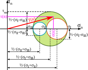
Figure 8: Mohr's circles for a three-dimensional state of stress. As can be seen in the picture, the three radii are calculated from the difference between two principal stresses.

The three-dimensional reality can be represented with 3 Mohr's circles of tension. There is an outer one that spans the plane of σ _Ⅲ and σ _I. Each traction vector must lie within the outer circle (or on the outer circle). Those stress combinations of normal stress and shear stress that lie within the inner circles cannot occur, which also means that there are only 3 normal stresses for which the shear stress is zero. In a state of stress where two principal stresses are zero, one circle degenerates to a point and the other inner circle is identical to the outer circle. In the case of a hydrostatic stress state, all three circles degenerate to one point, since there are no shear stresses and the same normal stress is present in every direction.

Determination of the normal vector or the traction vector

Figure 9: How to get the components of n constructively

Fig. 10: Construction of the Von Mises equivalent stress

One draws the three tension circles and the tension point (the point to which the traction vector T (n) should point) that is sought. This point must be between the three circles, if it lies exactly on a circle, the normal vector can be determined as with the 2D stress circle. A point of tension outside the outer circle or within one of the smaller circles cannot be assumed. By piercing in one of the three center points of the stress circles and subtracting the distance on one of the two circles with a different center point, you can determine double the angle to a main stress direction as in 2D . With this one can determine the normal vector:

${\displaystyle n=\cos(\alpha _{\mathrm {I} })\cdot n_{I}+\cos(\alpha _{\mathrm {II} })\cdot n_{II}+\cos(\alpha _{\mathrm {III} })\cdot n_{III}=}$ ${\displaystyle {\begin{pmatrix}\cos(\alpha _{\mathrm {I} }),\cos(\alpha _{\mathrm {II} }),\cos(\alpha _{\mathrm {III} })\end{pmatrix}}_{e_{I},e_{II},e_{III}}^{T}}$

It is sufficient to determine two angles and to determine the third via n² = cos² (α _I ) + cos² (α _Ⅱ ) + cos² (α _Ⅲ ). It is also possible to graphically determine the traction vector for a specific normal vector; here the steps mentioned above must be carried out in reverse order.

One side of an equilateral triangle is spanned by the main normal stresses σ _I and σ _III . The distance between the point of just spanned triangle does not lie on the abscissa, and σ _II corresponds to the von Mises equivalent stress .

Mohrscher Kreis: construction and evaluation

construction

Figure 11: Mohr's circle, principal stresses and principal stress directions for example ${\displaystyle {\begin{bmatrix}\sigma _{xx}&\tau _{xy}\\\tau _{xy}&\sigma _{yy}\end{bmatrix}}={\begin{bmatrix}-1&4\\4&5\end{bmatrix}}}$

---

The construction of the Mohr circle is done as shown in the adjacent picture according to the following scheme:

1. Drawing a map. Coordinate system for points . ${\displaystyle (t_{\bar {x}},t_{\bar {y}})}$
2. Enter the two points:
   • ${\displaystyle P_{0^{\circ }}=\left(t_{\bar {x}}(0^{\circ }),t_{\bar {y}}(0^{\circ })\right)=\left(\sigma _{xx},\tau _{xy}\right)}$
   • ${\displaystyle P_{90^{\circ }}=\left(t_{\bar {x}}(90^{\circ }),t_{\bar {y}}(90^{\circ })\right)=\left(\sigma _{yy},-\tau _{xy}\right)}$.

   Connect these two points with a straight line (dash-dotted line).

3. Draw the circle that contains the points and and the center of which is the intersection of the dash-dotted line with the axis. ${\displaystyle P_{0^{\circ }}}$ ${\displaystyle P_{90^{\circ }}}$ ${\displaystyle t_{\bar {x}}}$
4. Enter / read off the two points:
   • ${\displaystyle P_{\sigma _{\mathsf {max}}}=(\lambda _{1},0)}$
   • ${\displaystyle P_{\sigma _{\mathsf {min}}}=(\lambda _{2},0)}$

   Connect these two points with (blue dashed lines). ${\displaystyle P_{0^{\circ }}}$

5. Enter / read off the two points:
   • ${\displaystyle P_{\tau _{\mathsf {max}}}=(a,R)}$
   • ${\displaystyle P_{\tau _{\mathsf {min}}}=(a,-R)}$

   Connect these two points with (red dashed lines). ${\displaystyle P_{0^{\circ }}}$

evaluation

1. Cutting direction / cutting tension

Every point on the Mohr's circle in the figure in the construction section corresponds to an intersection angle , see figure 5 , on the one hand the angle between the x -axis and the normal unit vector n  - counting positively counterclockwise starting from x (in figure 5). On the other hand, in Mohr's circle, or the picture in the construction section , the angle between and the point that matches the respective cutting direction  - counting positively starting from clockwise. ${\displaystyle \varphi }$ ${\displaystyle \varphi }$ ${\displaystyle 2\varphi }$ ${\displaystyle P_{0^{\circ }}}$ ${\displaystyle (t_{\bar {x}},t_{\bar {y}})}$ ${\displaystyle P_{0^{\circ }}}$

For each predetermined cutting angle to read in Mohr's circle components of matching to this cutting direction average voltage vector from. These components are the pair that can be read at the point . ${\displaystyle \varphi }$ ${\displaystyle ({\bar {x}},{\bar {y}})}$ ${\displaystyle (t_{\bar {x}},t_{\bar {y}})}$ ${\displaystyle 2\varphi }$

2. Principal stresses

At the intersections of the circle with the axis are the components of the stress vectors or . The intersection stress vector t is therefore parallel to n at these intersection points , and therefore the principal stresses are or . ${\displaystyle t_{\bar {x}}}$ ${\displaystyle ({\bar {x}},{\bar {y}})}$ ${\displaystyle (t_{\bar {x}},t_{\bar {y}})=(\lambda _{1},0)}$ ${\displaystyle (t_{\bar {x}},t_{\bar {y}})=(\lambda _{2},0)}$ ${\displaystyle \lambda _{1}}$ ${\displaystyle \lambda _{2}}$

3. Principal directions of stress

The two associated main stress directions are perpendicular to each other. It is therefore sufficient to read off the corresponding direction. This is given by the cutting angle , i.e. H. half of the angle or the blue dashed line between and . This line / direction is the main stress direction. The direction in which the free cut is made is perpendicular to it. It is given by the blue dashed line between and . ${\displaystyle \lambda _{1}}$ ${\displaystyle \varphi _{1}}$ ${\displaystyle 2\varphi _{1}}$ ${\displaystyle (\lambda _{2},0)}$ ${\displaystyle P_{0^{\circ }}}$ ${\displaystyle (\lambda _{1},0)}$ ${\displaystyle P_{0^{\circ }}}$

4. Extreme values ​​of the shear stress

The radius of the circle is the greatest occurring shear stress, i.e. H.:

${\displaystyle {\begin{aligned}\tau _{\textsf {max}}&=t_{{\bar {y}}_{\textsf {max}}}=R\\\tau _{\textsf {min}}&=t_{{\bar {y}}_{\textsf {min}}}=-R\\\end{aligned}}}$

The corresponding intersection angles are offset by the intersection angles at which the principal stresses occur (see red dashed lines in the figure in the construction section ). ${\displaystyle 45^{\circ }}$

Special case: If the deviator part of the stress tensor is zero - i.e. i.e., if the stress tensor is a spherical tensor - the circle degenerates to a point. The following then applies to the components of the stress tensor in each coordinate system:

${\displaystyle {\begin{bmatrix}\sigma _{xx}&\tau _{xy}\\\tau _{xy}&\sigma _{yy}\end{bmatrix}}=\alpha {\begin{bmatrix}1&0\\0&1\end{bmatrix}}}$

Related topics

Mohr's distortion circles

Analogous to the Mohr stress circles, you can draw Mohr distortion circles that show you which states of distortion are assumed. However, there is no traction vector that specifies the stress components on any surface, as is the case with the stress circles.

Tensor components from two sections

Figure 12: Stress tensor components related to the coordinate system; Stress tensor components related to the rotated coordinate system for example ${\displaystyle (\sigma _{xx},\sigma _{yy},\tau _{xy})}$ ${\displaystyle (x,y)}$ ${\displaystyle (\sigma _{{\bar {x}}{\bar {x}}},\sigma _{{\bar {y}}{\bar {y}}},\tau _{{\bar {x}}{\bar {y}}})}$ ${\displaystyle \varphi }$ ${\displaystyle ({\bar {x}},{\bar {y}})}$ ${\displaystyle {\begin{bmatrix}\sigma _{xx}&\tau _{xy}\\\tau _{xy}&\sigma _{yy}\end{bmatrix}}={\begin{bmatrix}-1&4\\4&5\end{bmatrix}}}$

Let the stress tensor components be given with respect to the coordinate system. Let exactly one coordinate system be defined that is rotated by an angle with respect to the coordinate system, see the picture opposite. Let the stress tensor components be sought in relation to this one coordinate system . ${\displaystyle (x,y)}$ ${\displaystyle ({\bar {x}},{\bar {y}})}$ ${\displaystyle \varphi }$ ${\displaystyle (x,y)}$ ${\displaystyle ({\bar {x}},{\bar {y}})}$ ${\displaystyle (\sigma _{xx},\sigma _{yy},\tau _{xy})}$

Then these components can be determined by a cut under  - and a second cut under , because: ${\displaystyle \varphi }$ ${\displaystyle \varphi +90^{\circ }}$

${\displaystyle {\begin{aligned}{\begin{bmatrix}\sigma _{{\bar {x}}{\bar {x}}}\\\tau _{{\bar {x}}{\bar {y}}}\end{bmatrix}}&={\begin{bmatrix}t_{\bar {x}}(\varphi )\\t_{\bar {y}}(\varphi )\\\end{bmatrix}}\\{\begin{bmatrix}\tau _{{\bar {x}}{\bar {y}}}\\\sigma _{{\bar {y}}{\bar {y}}}\end{bmatrix}}&={\begin{bmatrix}-t_{\bar {y}}(\varphi +90^{\circ })\\t_{\bar {x}}(\varphi +90^{\circ })\\\end{bmatrix}}\\&={\begin{bmatrix}t_{\bar {y}}(\varphi )\\t_{\bar {x}}(\varphi +90^{\circ })\\\end{bmatrix}}\end{aligned}}}$

The last formulas make it possible to calculate the components of the stress tensor in relation to a coordinate system rotated by an angle . The functions and that are used to do this are the same as those used to construct Mohr's circle. And that's why you can read the components of the stress tensor in relation to a rotated coordinate system from Mohr's circle, see the picture at the beginning of this paragraph. ${\displaystyle \varphi }$ ${\displaystyle t_{\bar {x}}}$ ${\displaystyle t_{\bar {y}}}$

Tensor components from transformation relationship

These components of the stress tensor can also be calculated directly from the components of the stress tensor. The change in coordinates from to creates the following transformation relationship (also called push forward ) for the components of the (2,0) stress tensor: ${\displaystyle ({\bar {x}},{\bar {y}})}$ ${\displaystyle (x,y)}$ ${\displaystyle (x,y)}$ ${\displaystyle ({\bar {x}},{\bar {y}})}$

${\displaystyle {\begin{aligned}&{\begin{bmatrix}\sigma _{{\bar {x}}{\bar {x}}}&\tau _{{\bar {x}}{\bar {y}}}\\\tau _{{\bar {x}}{\bar {y}}}&\sigma _{{\bar {y}}{\bar {y}}}\end{bmatrix}}\\=&{\begin{bmatrix}c_{\varphi }&s_{\varphi }\\-s_{\varphi }&c_{\varphi }\\\end{bmatrix}}{\begin{bmatrix}\sigma _{xx}&\tau _{xy}\\\tau _{xy}&\sigma _{yy}\\\end{bmatrix}}{\begin{bmatrix}c_{\varphi }&-s_{\varphi }\\s_{\varphi }&c_{\varphi }\\\end{bmatrix}}\\=&{\begin{bmatrix}c_{\varphi }\sigma _{xx}+s_{\varphi }\tau _{xy}&c_{\varphi }\tau _{xy}+s_{\varphi }\sigma _{yy}\\-s_{\varphi }\sigma _{xx}+c_{\varphi }\tau _{xy}&-s_{\varphi }\tau _{xy}+c_{\varphi }\sigma _{yy}\\\end{bmatrix}}{\begin{bmatrix}c_{\varphi }&-s_{\varphi }\\s_{\varphi }&c_{\varphi }\\\end{bmatrix}}\\=&{\begin{bmatrix}(c_{\varphi }\sigma _{xx}+s_{\varphi }\tau _{xy})c_{\varphi }+(c_{\varphi }\tau _{xy}+s_{\varphi }\sigma _{yy})s_{\varphi }&(c_{\varphi }\sigma _{xx}+s_{\varphi }\tau _{xy})(-s_{\varphi })+(c_{\varphi }\tau _{xy}+s_{\varphi }\sigma _{yy})c_{\varphi }\\(-s_{\varphi }\sigma _{xx}+c_{\varphi }\tau _{xy})c_{\varphi }+(-s_{\varphi }\tau _{xy}+c_{\varphi }\sigma _{yy})s_{\varphi }&(-s_{\varphi }\sigma _{xx}+c_{\varphi }\tau _{xy})(-s_{\varphi })+(-s_{\varphi }\tau _{xy}+c_{\varphi }\sigma _{yy})c_{\varphi }\\\end{bmatrix}}\\=&{\begin{bmatrix}(\sigma _{xx}c_{\varphi }+\tau _{xy}s_{\varphi })c_{\varphi }+(\tau _{xy}c_{\varphi }+\sigma _{yy}s_{\varphi })s_{\varphi }&-(\sigma _{xx}c_{\varphi }+\tau _{xy}s_{\varphi })s_{\varphi }+(\tau _{xy}c_{\varphi }+\sigma _{yy}s_{\varphi })c_{\varphi }\\-(\sigma _{xx}c_{\varphi }+\tau _{xy}s_{\varphi })s_{\varphi }+(\tau _{xy}c_{\varphi }+\sigma _{yy}s_{\varphi })c_{\varphi }&(\sigma _{xx}c_{\varphi +{\tfrac {\pi }{2}}}+\tau _{xy}s_{\varphi +{\tfrac {\pi }{2}}})c_{\varphi +{\tfrac {\pi }{2}}}+(\tau _{xy}c_{\varphi +{\tfrac {\pi }{2}}}+\sigma _{yy}s_{\varphi +{\tfrac {\pi }{2}}})s_{\varphi +{\tfrac {\pi }{2}}}\\\end{bmatrix}}\end{aligned}}}$

Comparison with the equations for and from section # (n, m) components yields: ${\displaystyle t_{\bar {x}}}$ ${\displaystyle t_{\bar {y}}}$

${\displaystyle {\begin{aligned}{\begin{bmatrix}\sigma _{{\bar {x}}{\bar {x}}}&\tau _{{\bar {x}}{\bar {y}}}\\\tau _{{\bar {x}}{\bar {y}}}&\sigma _{{\bar {y}}{\bar {y}}}\end{bmatrix}}&={\begin{bmatrix}t_{\bar {x}}(\varphi )&t_{\bar {y}}(\varphi )\\t_{\bar {y}}(\varphi )&t_{\bar {x}}\left(\varphi +{\tfrac {\pi }{2}}\right)\end{bmatrix}}\end{aligned}}}$

This result is equivalent to the result from the last section, see also the picture in the paragraph Tensor components from two sections .

Often this result is also written as:

${\displaystyle {\begin{aligned}\sigma _{{\bar {x}}{\bar {x}}}(\varphi )&={\tfrac {1}{2}}(\sigma _{xx}+\sigma _{yy})+{\tfrac {1}{2}}(\sigma _{xx}-\sigma _{yy})c_{2\varphi }+\tau _{xy}s_{2\varphi }\\\tau _{{\bar {x}}{\bar {y}}}(\varphi )&=-{\tfrac {1}{2}}(\sigma _{xx}-\sigma _{yy})s_{2\varphi }+\tau _{xy}c_{2\varphi }\end{aligned}}}$

Conversion of geometrical moments of inertia

Figure 13: Mohr's circle of inertia, main moments of inertia for example ${\displaystyle I_{1},I_{2}}$ ${\displaystyle {\begin{bmatrix}I_{y}&I_{yz}\\I_{yz}&I_{z}\end{bmatrix}}={\begin{bmatrix}3&4\\4&9\end{bmatrix}}}$

The transformation rule for geometrical moments of inertia can be determined exactly like the transformation rule for the components of the stress tensor. The stress tensor is a linear mapping between vectors according to:

${\displaystyle {\begin{aligned}{\begin{bmatrix}t_{x}\\t_{y}\end{bmatrix}}&={\begin{bmatrix}\sigma _{xx}&\tau _{xy}\\\tau _{xy}&\sigma _{yy}\\\end{bmatrix}}{\begin{bmatrix}n_{x}\\n_{y}\end{bmatrix}}\\{\begin{bmatrix}t_{\bar {x}}\\t_{\bar {y}}\end{bmatrix}}&={\begin{bmatrix}\sigma _{{\bar {x}}{\bar {x}}}&\tau _{{\bar {x}}{\bar {y}}}\\\tau _{{\bar {x}}{\bar {y}}}&\sigma _{{\bar {y}}{\bar {y}}}\end{bmatrix}}{\begin{bmatrix}n_{\bar {x}}\\n_{\bar {y}}\end{bmatrix}}\end{aligned}}}$

In order for these maps to apply regardless of the choice of coordinate system, the components of the stress tensor must meet the following transformation rules:

${\displaystyle {\begin{aligned}{\begin{bmatrix}\sigma _{{\bar {x}}{\bar {x}}}&\tau _{{\bar {x}}{\bar {y}}}\\\tau _{{\bar {x}}{\bar {y}}}&\sigma _{{\bar {y}}{\bar {y}}}\end{bmatrix}}&={\begin{bmatrix}c_{\varphi }&s_{\varphi }\\-s_{\varphi }&c_{\varphi }\\\end{bmatrix}}{\begin{bmatrix}\sigma _{xx}&\tau _{xy}\\\tau _{xy}&\sigma _{yy}\\\end{bmatrix}}{\begin{bmatrix}c_{\varphi }&-s_{\varphi }\\s_{\varphi }&c_{\varphi }\\\end{bmatrix}}\end{aligned}}}$

Completely analogously, for a profile bar, between bending moments and curvatures (based on the neutral axis) with the area moments of inertia is defined as ${\displaystyle M_{y},M_{z}}$ ${\displaystyle \psi _{y},\psi _{z}}$

${\displaystyle {\begin{aligned}I_{y}&=\int z^{2}dA\\I_{z}&=\int y^{2}dA\\I_{yz}&=-\int yzdA\\\end{aligned}}}$

the linear relationship:

${\displaystyle {\begin{aligned}{\begin{bmatrix}M_{y}\\M_{z}\end{bmatrix}}&={\begin{bmatrix}EI_{y}&EI_{yz}\\EI_{yz}&EI_{z}\\\end{bmatrix}}{\begin{bmatrix}\psi _{y}\\\psi _{z}\end{bmatrix}}\\{\begin{bmatrix}M_{\bar {y}}\\M_{\bar {z}}\end{bmatrix}}&={\begin{bmatrix}EI_{\bar {y}}&EI_{{\bar {y}}z}\\EI_{{\bar {y}}{\bar {z}}}&EI_{\bar {z}}\\\end{bmatrix}}{\begin{bmatrix}\psi _{\bar {y}}\\\psi _{\bar {z}}\end{bmatrix}}\end{aligned}}}$

The moments and the curvatures transform like pseudo vectors - i.e. like vectors when the coordinate system is rotated. And that is why the transformation rule for the area moments of inertia is:

${\displaystyle {\begin{aligned}{\begin{bmatrix}EI_{\bar {y}}&EI_{{\bar {y}}{\bar {z}}}\\EI_{{\bar {y}}{\bar {z}}}&EI_{\bar {z}}\\\end{bmatrix}}&={\begin{bmatrix}c_{\varphi }&s_{\varphi }\\-s_{\varphi }&c_{\varphi }\\\end{bmatrix}}{\begin{bmatrix}EI_{y}&EI_{yz}\\EI_{yz}&EI_{z}\\\end{bmatrix}}{\begin{bmatrix}c_{\varphi }&-s_{\varphi }\\s_{\varphi }&c_{\varphi }\\\end{bmatrix}}\\\Leftrightarrow {\begin{bmatrix}I_{\bar {y}}&I_{{\bar {y}}{\bar {z}}}\\I_{{\bar {y}}{\bar {z}}}&I_{\bar {z}}\\\end{bmatrix}}&={\begin{bmatrix}c_{\varphi }&s_{\varphi }\\-s_{\varphi }&c_{\varphi }\\\end{bmatrix}}{\begin{bmatrix}I_{y}&I_{yz}\\I_{yz}&I_{z}\\\end{bmatrix}}{\begin{bmatrix}c_{\varphi }&-s_{\varphi }\\s_{\varphi }&c_{\varphi }\\\end{bmatrix}}\end{aligned}}}$

Mohr's circle can also be used to convert the area moments of inertia when changing coordinates and to convert the components of the stress tensor.

Program to try out

Fig. 14: Plot of some pairs , generated with the program shown here ${\displaystyle (t_{\bar {x}},t_{\bar {y}})}$

with Matplotlib and NumPy

import matplotlib.pyplot as plt
from numpy import pi, sin, cos, array, transpose, dot
from numpy import radians, degrees, set_printoptions

#There is the (x,y)-system and the (X,Y)-system.

#         [s_xx  t_xy ]     [-1  4 ]
#  S_xy = [           ]  =  [      ]
#         [t_xy  s_yy ]     [ 4  5 ]

# ---
# --- User input:
# ---

# 1: Stress tensor components:
(s_xx, s_yy, t_xy) = (-1, 5, 4)

# 2: List of angles phi in degrees:
phi_deg = array( [0., 30., 60., 90., 120., 150.] )

# ---
# --- Program output:
# ---

# phi [ t_X, t_Y ]

# 0.0  [-1.   4.  ]
# 30.0 [ 3.96 4.6 ]
# 60.0 [ 6.96 0.6 ]
# ...

# phi [ s_XX, t_XY ]
#     [ t_XY, s_YY ]

# 0.0   [-1.   4.  ]
#       [ 4.   5.  ]
# 30.0  [ 3.96 4.6 ]
#       [ 4.6  0.04]
# 60.0  [ 6.96 0.6 ]
#       [ 0.6 -2.96]
# ...

# ---
# --- Program:
# ---

# Matrix of components::
S_xy = array([ [s_xx, t_xy],
               [t_xy, s_yy] ])

# Yes
half = 0.5
two  = 2.0

# Some functions for later use:
def c2(phi):
    """ computes cos(2 phi) """
    return cos(two*phi)

def s2(phi):
    """ computes sin(2 phi) """
    return sin(two*phi)

def get_t_X(phi):
    """
    computes t_X(phi) as in section
    "(X,Y)-Komponenten"
    """
    t_X = half*(s_xx + s_yy) + half*(s_xx - s_yy) * c2(phi) + t_xy*s2(phi)
    return t_X

def get_t_Y(phi):
    """
    computes t_Y(phi) as in section
    "(X,Y)-Komponenten"
    """
    t_Y = -half*(s_xx - s_yy) * s2(phi) + t_xy * c2(phi)
    return t_Y

def get_t_XY(phi):
    """
    computes pair (t_X, t_Y)
    """
    t_X = get_t_X(phi)
    t_Y = get_t_Y(phi)
    return array([t_X, t_Y])

def get_R(phi):
    """
    computes rotation matrix as in section
    "Tensorkomponenten aus Transformationsbeziehung"
    """
    Rt = array([ [ cos(phi), sin(phi)],
                 [-sin(phi), cos(phi)] ] )
    return Rt

def get_S_XY(phi):
    """
    computes S_XY = R * S_xy * R^T as in section
    "Tensorkomponenten aus Transformationsbeziehung"
    """
    R = get_R(phi)
    R_T = R.transpose()
    S_XY = dot( dot(R, S_xy), R_T )
    return S_XY

# Compute and plot some pairs (t_X, t_Y):

# phi in radians:
phis = array( [ radians(a) for a in phi_deg ] )

# for prettier printing:
set_printoptions(precision=2)

print ()
print ("phi   [ t_X, t_Y ]")
print ()
for phi in phis:
    tX_tY = get_t_XY(phi)
    print (degrees(phi),"  ", tX_tY)

print ()
print ("phi   [ s_XX, t_XY ]")
print ("      [ t_XY, s_YY ]")
print ()
for phi in phis:
    S_XY = get_S_XY(phi)
    print (degrees(phi), "  ", S_XY[0])
    print ("       ",         S_XY[1])

# Now plot these pairs (t_X, t_Y):

# phi --> t_X(phi):
t_X = list(map(get_t_X, phis))
# phi --> t_Y(phi):
t_Y = list(map(get_t_Y, phis))

# color = phi in degrees:
color = degrees(phis)

# make the circle be a circle:
plt.axis("equal")

# plot some colored points:
plt.scatter(t_X, t_Y, s=100, c=color)

# add colorbar:
cbar = plt.colorbar()

# plt.clim(0,180.)
# add ticks to colorbar:
cbar.set_ticks(degrees(phis))

# show plot:
plt.show()

literature

• Gross, Hauger, Schröder, Wall: Technical Mechanics 2 . 12th edition. Springer Vieweg, 2012, ISBN 978-3-642-40965-3 .
• F. Jung: The Culmann and the Mohr circles. In: Austrian engineering archive. 1, No. 4-5, 1946/47, ISSN  0369-7819 , pp. 408-410.
• Istvan Szabo : Introduction to Engineering Mechanics. Springer, 1984, ISBN 3-540-13293-7 .
• Jerrold E. Marsden , Thomas JR Hughes : Mathematical Foundations of Elasticity. 1994, ISBN 0-486-67865-2 .
• Otto Mohr : Treatises from the field of technical mechanics. 3rd ext. Ed. v. K. Beyer, H. Spangenberg. Ernst & Son, Berlin 1928
• Walter Noll , Clifford Truesdell : The Non-Linear Field Theories of Mechanics. Springer-Verlag, New York 1965, ISBN 3-540-02779-3 .
• Walter Noll: Foundations of Mechanics and Thermodynamics, Selected Papers. Springer-Verlag, New York 1974, ISBN 0-387-06646-2 .
• Stephen P. Timoshenko , James Norman Goodier : Theory of Elasticity . 3. Edition. McGraw-Hill International Editions, 1970, ISBN 0-07-085805-5 .
• Stephen P. Timoshenko: History of strength of materials: with a brief account of the history of theory of elasticity and theory of structures (=  Dover Books on Physics ). Dover Publications, 1983, ISBN 0-486-61187-6 .
• Johannes Wiedemann: Lightweight Construction, Volume 1: Elements . Springer, 1986, ISBN 3-540-16404-9 .
• Christian Spura: Technical Mechanics 2. Elastostatics . Springer, 2019, ISBN 978-3-658-19978-4 .

Individual evidence

1. ^ Mohr, Civilingenieur 1882, p. 113, after Timoshenko, History of strength of materials, McGraw Hill 1953, p. 285
2. ^ Karl-Eugen Kurrer , History of Structural Analysis. In Search of Balance , Ernst & Sohn 2016, p. 323
3. ^ Johannes Wiedemann: Lightweight construction. Vol. 1: Elements.

Web links

Commons : Mohr's circle  - collection of images, videos and audio files

• Visualization of symmetrical tensors with superquadrics