
Dijkstra's algorithm


The Dijkstra's algorithm (after its inventor Edsger W. Dijkstra ) is an algorithm of the class of greedy algorithms and solves the problem of the shortest paths for a given starting node. It thus calculates a shortest path between the given starting node and one of the (or all) other nodes in an edge-weighted graph (provided that this does not contain any negative edges).
For disconnected undirected graphs, the distance to those nodes to which there is no path from the start node is infinite. The same applies to directed graphs that are not strongly connected .
algorithm
Informal representation
The basic idea of the algorithm is to always follow the edge that promises the shortest route section from the start node. Other edges are only followed when all shorter route sections have been taken into account. This procedure ensures that when a node is reached, there cannot be a shorter path to it. A distance calculated once between the starting node and a visited node is no longer changed. Distances to nodes that have not yet been processed, on the other hand, can change during the course of the algorithm, namely decrease. This procedure is continued until the distance to the destination node has been calculated ( single-pair shortest path ) or the distances from all nodes to the start node are known ( single-source shortest path ).

The algorithm can be described by the following steps. Both the shortest routes and their node sequences are calculated.
- Assign the two properties "Distance" and "Predecessor" to all nodes. Initialize the distance in the starting node with 0 and in all other nodes with .
- As long as there are still unvisited nodes, select the one with the minimum distance and
- Remember that this node has already been visited.
- Calculate the sum of the respective edge weight and the distance in the current node for all neighboring nodes that have not yet been visited.
- If this value for a node is smaller than the distance saved there, update it and set the current node as the predecessor.
- This step is also known as update or relaxation / relaxation .

In this form, the algorithm calculates the shortest paths to all other nodes based on a starting node. If, on the other hand, you are only interested in the route to a very specific node, you can stop in step (2) when the node you are looking for is the active one.

The Dijkstra algorithm is one of the greedy algorithms that prefer the currently most promising partial solution in each step due to the fact that once the distances to the start node cannot be changed. Unlike some other greedy algorithms, the Dijkstra algorithm always calculates an optimal solution. This property is based on the assumption that the shortest sections between nodes in a path together form the shortest path on this path. Assuming positive edge weights, the assumption is valid, because if a shorter path from the start node to a destination node were found, one would have had to examine its shorter section earlier in order to carry out the algorithm correctly. Then you would have found the destination node earlier on the shorter section than on the longer route.
However, the assumption is no longer true if the graph contains negative edge weights. Then each partial route can be a shortest route between the endpoints, but the total distance could be improved over a longer partial route if a negative edge reduces the route length again. In the picture with nodes 1, 2, 3 and 4, the Dijkstra algorithm would find the shortest path from 1 to 3 via 2, since the step to 4 is overall longer than the entire upper path. The negative edge causes the lower path to be shorter.
Algorithm in pseudocode
The following lines of pseudocode describe a function called Dijkstra that takes a graph and a start node in the graph as input. The starting node indicates the node from which the shortest paths to all nodes are sought. The result is a list that specifies for each node v the previous node on the way from the start node to v .
The graph consists of nodes and weighted edges between its nodes. If there is an edge between two nodes, they are each neighbors. The node currently under consideration in the sub-step is denoted by u and is called the “ consideration node ”. The possible, upcoming neighboring nodes are referred to as “test nodes” in the respective upcoming interim investigation with v . The edge weight between the observation node u and the respective test node v is specified in the pseudocode as distance_between (u, v) .
The numerical value of distance [v '] contains the respective total distance in the investigation branch, which adds up the partial distances from the starting point via possible intermediate nodes and the current node u to the next node v' to be investigated .
First, the distances and predecessors are initialized depending on the graph and starting node. This is done in the initialize method . The actual algorithm uses a method distance_update, which updates the distances if a shorter path is found.
 1  Funktion Dijkstra(Graph, Startknoten):
 2      initialisiere(Graph,Startknoten,abstand[],vorgänger[],Q)
 3      solange Q nicht leer:                       // Der eigentliche Algorithmus
 4          u:= Knoten in Q mit kleinstem Wert in abstand[]
 5          entferne u aus Q                                // für u ist der kürzeste Weg nun bestimmt
 6          für jeden Nachbarn v von u:
 7              falls v in Q:                            // falls noch nicht berechnet
 8                 distanz_update(u,v,abstand[],vorgänger[])   // prüfe Abstand vom Startknoten zu v
 9      return vorgänger[]
The initialization sets the distances to infinite and the predecessors as unknown. Only the starting node has the distance 0. The set Q contains the nodes to which a shortest path has not yet been found.
 1  Methode initialisiere(Graph,Startknoten,abstand[],vorgänger[],Q):
 2      für jeden Knoten v in Graph:
 3          abstand[v]:= unendlich
 4          vorgänger[v]:= null
 5      abstand[Startknoten]:= 0
 6      Q:= Die Menge aller Knoten in Graph
The distance from the starting node to the node v is shortened if the path to v via u is shorter than the previously known path. Accordingly, u becomes the predecessor of v by the shortest route.
 1  Methode distanz_update(u,v,abstand[],vorgänger[]):
 2      alternativ:= abstand[u] + abstand_zwischen(u, v)   // Weglänge vom Startknoten nach v über u
 3      falls alternativ < abstand[v]:
 4          abstand[v]:= alternativ
 5          vorgänger[v]:= u
If you are only interested in the shortest path between two nodes, you can have the algorithm abort after line 5 of the Dijkstra function if u = the destination node .
The shortest path to a target node can now be determined by iterating over the previous ones :
1  Funktion erstelleKürzestenPfad(Zielknoten,vorgänger[])
2   Weg[]:= [Zielknoten]
3   u:= Zielknoten
4   solange vorgänger[u] nicht null:   // Der Vorgänger des Startknotens ist null
5       u:= vorgänger[u]
6       füge u am Anfang von Weg[] ein
7   return Weg[]
implementation
Nodes and edges between nodes can usually be represented by matrices or pointer structures. A pointer can also refer to the predecessor of a node. The distances between the nodes can be saved in fields .
For an efficient implementation, the set Q of the nodes for which the shortest path has not yet been found is implemented by a priority queue . The complex initialization only takes place once, but repeated accesses to Q are more efficient. The key value for the node is its respective distance, which is specified in the pseudocode with distance [v] . If the distance becomes shorter, the queue must be partially re-sorted.
A distance table or an adjacency matrix can be used as a data structure for this .
example
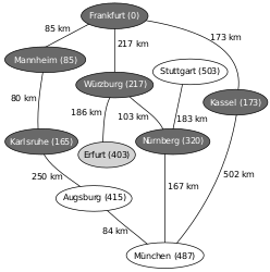
An example of the application of Dijkstra's algorithm is the search for a shortest path on a map. In the example used here, you want to find a shortest path from Frankfurt to Munich in the map of Germany shown below .
The numbers on the connections between two cities indicate the distance between the two cities connected by the edge. The numbers behind the city names indicate the calculated distance from the city to the starting point in Frankfurt, where ∞ stands for an unknown distance. The nodes highlighted in light gray are the nodes whose distance is relaxed (i.e. shortened if a shorter route has been found), the nodes highlighted in dark gray are those to which the shortest route from Frankfurt is already known.
The next neighbor is selected according to the principle of a priority queue. Relaxed distances therefore require a re-sorting.
- example

Initial situation: non-initialized graph with starting node Frankfurt and destination node Munich

Determine distances from the starting node (Frankfurt) ( relaxation ), re-sort the priority queue Q (1. Mannheim, 2. Kassel, 3. Würzburg, ...)

Mannheim is the closest node, relaxation with the neighboring node Karlsruhe, the next predecessor of Karlsruhe is now Mannheim, re-sorting of Q (1. Karlsruhe, 2. Kassel, 3. Würzburg, ...)

According to Q, the node to be examined closest to the starting point is now Karlsruhe, relaxation with Augsburg, re-sorting of Q (1. Kassel, 2. Würzburg, 3. Augsburg, ...)

The closest node to be examined is now Kassel, relaxation with Munich, re-sorting of Q (1. Würzburg, 2. Augsburg, 3. Munich, ...)

The closest node to be examined is now Würzburg, relaxation with Erfurt and Nuremberg, re-sorting of Q (1. Nuremberg, 2. Erfurt, 3. Augsburg, 4. Munich, ...)

The closest node to be examined is now Nuremberg, relaxation with Munich and Stuttgart, re-sorting of Q (1. Erfurt, 2. Augsburg, 3. Munich, 4. Stuttgart, ...)
The closest node to be examined is now Erfurt, relaxation with nobody, re-sorting of Q (1. Augsburg, 2. Munich, 3. Stuttgart, ...)

The closest node to be examined is now Augsburg, relaxation with Munich, re-sorting of Q (1st Munich, 2nd Stuttgart ...)

The destination node is to be examined: The shortest route to Munich is now known; Reconstruction using createShortestPath () . This is: Frankfurt-Würzburg-Nuremberg-Munich.


Basic concepts and relationships
An alternative algorithm for finding the shortest paths, which is based on Bellman's principle of optimality , is the Floyd-Warshall algorithm . The principle of optimality states that if the shortest path from A to C leads via B, partial path A B must also be the shortest path from A to B.
Another alternative algorithm is the A * algorithm , which extends Dijkstra's algorithm by an estimation function. If this fulfills certain properties, the shortest path can be found more quickly under certain circumstances.
There are different acceleration techniques for the Dijkstra algorithm, for example Arcflag .
Calculation of a spanning tree

After the end of the algorithm is in the predecessor pointers π a partial spanning tree of the component of from shortest paths from all nodes of the component taken in the queue records. However, this tree is not necessarily minimal, as the figure shows:

Let be a number greater than 0. Trees with minimal spans are given either by the edges and or and . The total cost of a minimally exciting tree is . Dijkstra's algorithm delivers the edges with starting point and as a result. The total cost of this exciting tree is .


The calculation of a minimum spanning tree is possible with the algorithm from Prim or the algorithm from Kruskal .
Time complexity
The following estimate only applies to graphs that do not contain negative edge weights.
The runtime of the Dijkstra algorithm depends on the number of edges and the number of nodes . The exact time complexity depends on the data structure in which the nodes are stored. The following applies to all implementations of :


where and stand for the complexity of the decrease-key and extract-minimum operations . The simplest implementation for is a list or an array. Here is the time complexity .


Normally, you will fall back on a priority queue by using the nodes there as elements with their respective previous distance as key / priority.
The optimal runtime for a graph is by using a Fibonacci heap for the Dijkstra algorithm.


Applications
Route planners are a prominent example where this algorithm can be used. The graph represents the traffic route network that connects different points with each other. You are looking for the shortest route between two points.
Some topological indices , such as Balaban's J-index , require weighted distances between the atoms of a molecule . The weighting in these cases is the binding order.
Dijkstra's algorithm is also used on the Internet as a routing algorithm in the OSPF , IS-IS and OLSR protocol. The latter Optimized Link State Routing protocol is a version of Link State Routing adapted to the requirements of a mobile wireless LAN . It is important for mobile ad hoc networks . One possible application of this is in free radio networks .
The Dijkstra algorithm can also be used to solve the coin problem , a number-theoretic problem that at first glance has nothing to do with graphs.
Other methods for calculating shortest paths
If one has enough information about the edge weights in the graph to be able to derive a heuristic for the costs of individual nodes, it is possible to extend Dijkstra's algorithm to the A * algorithm . In order to calculate all shortest paths from one node to all other nodes in a graph, one can also use the Bellman-Ford algorithm , which can deal with negative edge weights. The Floyd and Warshall algorithm finally computes the shortest paths of all nodes to one another.
literature
- Thomas H Cormen, Charles E. Leiserson , Ronald L. Rivest , Clifford Stein: Algorithms - An Introduction . Oldenbourg, Munich, Vienna 2004, ISBN 3-486-27515-1 , pp. 598–604 (Original title: Introduction to algorithms . Translated by Karen Lippert, Micaela Krieger-Hauwede).
- Edsger W. Dijkstra : A note on two problems in connexion with graphs. In: Numerical Mathematics. 1, 1959, pp. 269-271; ma.tum.de (PDF; 739 kB).
Web links
- Python implementation with explanations
- Implementation in the free Python - Library NetworkX
- Interactive applet for learning, trying out and demonstrating the algorithm
- Java applet for Dijkstra (English)
- Interactive visualization and animation of Dijkstra's algorithm, suitable for people with no prior knowledge of algorithms (English)
- Implementation in C (English)
- Explanation based on an analog model (PDF; 213 kB)
- Public Software Library in Java with this and other algorithms (english)
- Java implementation - simulation / evaluation (English)
- Dijkstra's algorithm in C # (csharp). ( Memento from February 11, 2013 in the web archive archive.today ).
Individual evidence
- ↑ Tobias Häberlein: Practical Algorithms with Python. Oldenbourg, Munich 2012, ISBN 978-3-486-71390-9 , p. 162 ff.
- ^ The Simple, Elegant Algorithm That Makes Google Maps Possible. At: VICE. Retrieved March 24, 2015.
- ^ Thomas H. Cormen: Introduction to Algorithms . MIT Press, S. 663 .