
Trade equilibrium
The trade equilibrium is understood to be an interstate exchange equilibrium . This is the case when the import and export of an economy are of equal value. The trade equilibrium leads to the equilibrium of the trade balance in the national accounts , which then shows neither a debit nor a credit balance.
As long as there is trade equilibrium, the entire foreign trade of an economy can be imagined as an exchange in kind of all exported goods for all imported goods. Imports and exports cause the flow of money to run counter to the flow of goods. However, since import and export are worth the same, created by balance neither a flow of funds into the economy under consideration, nor a cash outflow from the economy under observation.
Standard model of a trading economy
The standard model , which is used to analyze real problems, is a merger of the Ricardo model and the Heckscher-Ohlin model. This combination of the two individual models is due to the fact that they mask out certain parts of reality and make different assumptions about the production possibilities.
Relevant theories
Ricardo model
The Ricardo model deals with the comparative advantage , but does not allow any statements about the income distribution . The production possibilities are determined by the assignment of the work to the different areas.
Heckscher-Ohlin model
The Heckscher-Ohlin model looks at the effect of trade on income distribution. This effect is caused by various production factors that cause differences in resources and thus influence the structure of trade.
Similarities between the two models
Although the two theories differ, they have common features that can be interpreted as characteristics of the standard model of a trading world economy . Therefore, both theories can be understood as special cases of the Standard Model.
The common features of both models and thus the features of the standard model are, on the one hand, that the production capacity of an economy can be represented by transformation curves and the differences in their course are the cause of trade. On the other hand the production possibilities determine the relative supply structure of a country. A final commonality of the two theories is that the world trade equilibrium, which lies between the national relative supply curves, is determined by the relative world demand and the relative world supply.
Characteristics of the trade balance
The properties of trade equilibrium include various patterns of specialization, trade restrictions, and welfare effects.
Pattern of specialization
The properties of the trade equilibrium relate to different patterns of specialization, which represent the main focal points of the model. According to Paul R. Krugman and Maurice Obstfeld , the trade balance relates to the:
- Relationship between transformation curve and supply curve,
- Relationship between relative prices and relative demand,
- Determination of the world equilibrium through the relative world supply and the relative world demand
- Impact of the terms of trade on a country's welfare.
Equality of exports and imports
Another specialization pattern of this model is the matching of exports and imports , which depends on the price relationships. As a result, goods that are produced domestically must correspond exactly to imports from abroad. Conversely, the import of the other good must be equivalent to the export from abroad.
Comparative cost advantage The model of the comparative cost advantage, which goes back to David Ricardo as part of the Ricardo model, represents a specialization pattern in the sense of the properties of the trade equilibrium. The comparative cost advantage here has the character of a complete specialization, so that with two countries in the model each country exactly a good is produced and exported.
Trade barriers
The second property is the effect of trade barriers . Trade barriers such as import tariffs or export subsidies are usually not introduced in order to change a country's terms of trade . Rather, these state interventions support the distribution of income, serve to promote important industries and actually affect trade. The characteristics of both are distinguished in that they cause a price difference.
duties
Customs duties are charges that are levied when goods are imported ( import duty ) or when goods are exported ( export duty ). When an import duty is levied, the price increases domestically in contrast to abroad. The direct effect of an import duty is that it makes imported goods more expensive domestically than abroad. In doing so, he promotes domestic production.
Export subsidies
In addition, export subsidies are payments to domestic producers who sell their goods abroad without the companies demanding anything in return. This form of trade barriers is particularly intended to support industries that have problems on the market.
As a result, subsidies represent a state subsidy payment. The price obtained by the seller exceeds the payment made by the customer. The difference between the two values is regarded as a subsidy . The direct effect of export subsidies manifests itself in an export incentive for producers. Because as long as the domestic price is not higher, selling abroad seems more advantageous. The export subsidies consequently increase the price of the good domestically.
By changing the price of both trade barriers, supply and demand are changed. At the same time, this also changes the terms of trade and, accordingly, welfare.
Welfare effects
Welfare
Welfare is the sum of consumer surplus and producer surplus , that is, the profit or the benefit of the producer or the consumer.
Consumer surplus
A so-called consumer surplus is the difference between the value that a good has and the price one has to pay for it. This definition can be illustrated with a simple example: if you take bread that has a personal value of 5 euros, if you buy this bread for 3 euros, the consumer surplus is 2 euros.
Producer surplus
The situation is similar with the producer surplus. It represents the difference between the money that the seller receives for selling a good and the costs that the seller had to manufacture and sell that good. Using the example of bread, this can be illustrated as follows: The seller sells the bread for 3 euros, its production costs amount to 1 euro. He has thus achieved a producer pension of 2 euros.
Example of welfare in economics "A" and "B"
Using the model of an economy, the following fictitiously chosen example can be constructed on the subject of welfare.
| Name of the economy | Producing good 1 | producing good 2 |
|---|---|---|
| A. | textiles | Food |
| B. | Food | textiles |
Economy "A" only exports textiles to Economy "B", which Economy "A" is able to do due to its innovative production processes. The productivity of textile production increases accordingly. Economy “A” therefore increasingly prefers the production of textiles compared to food production. In the case of the “A” economy, there is growth. As a further consequence, “A” imports food from the “B” economy. The effects of growth on economy "A" amount to four effects:
- The transformation curve shifts in the direction of the textiles.
- Relative prices are falling as more and more textiles are available compared to demand.
- The terms of trade, that is, the relationship between the prices of exports and imports, decrease when the relative prices fall.
- Worsening terms of trade reduce welfare.
In the case of economy “B”, this sequence is analogous, only there are different effects. Economy "B" exports food and imports textiles. It thus benefits from the specialization of the “A” national economy by being able to achieve a favorable price for the textiles when importing. This lower price is due to the high range of textiles that national economy “A” can make available through its specialized production process.
In the case of economy “B” there is therefore an opposite growth to economy “A”. The effects of this growth on economy "B" amount to four relationships:
- The transformation curve shifts in the direction of the textiles.
- Relative prices are falling as more and more textiles are available compared to demand
- The terms of trade rise as the relative prices fall.
- Welfare increases as the terms of trade improve.
A trade equilibrium develops as a result, provided that the values of exports and imports (terms of trade) are equal and, in particular, imports correspond to exports and vice versa. A new trade equilibrium can come about, provided that every relationship can compensate each other. As a result, the demand for textiles is falling again, so the supply and consequently also the price are falling. The values would strive for a new equilibrium.
General Effects of Welfare
General:
| Effect of export price | Effect welfare |
|---|---|
| The export price rises | Welfare increases |
| The export price drops | Welfare declines |
| The import price drops | Welfare increases |
| The import price rises | Welfare declines |
Derivation of the relative price in equilibrium for foreign trade
Premises

Several assumptions or premises apply to the derivation of the relative price in equilibrium for foreign trade. It is assumed that the existing world economy consists of two countries. Here the domestic exports textiles and the foreign exports food. This is only one example of goods that an economy can focus on and serves to explain the facts. Furthermore, we assume trade samples that have different production capacities in Germany and abroad. These trading patterns are represented by the relative supply curves in the figure.
In addition, both countries have the same preferences in terms of demand. This leads to an identical relative demand curve. The demand of both countries for the respective good (here textiles and food) is included in the relative world demand. The relative world demand arises mathematically as follows: (D C + D A C ) / (D F + D A F ). D C stands for the demand for textiles at home, D A C stands for the demand for textiles abroad, D F stands for the demand for food at home and D A F stands for the demand for food abroad. Due to the identical preferences of both countries, the relative demand curve overlaps with the curves of the relative demand of the individual countries.
At any given relative price P C / P F, the home country produces textiles (Q C ) and food (Q F ). This assumption also applies to foreign countries, with textiles being designated as Q A C and food as Q A F for foreign countries . However, the following always applies: Q C / Q F > Q A C / Q A F If you calculate the sums of the output quantities for textiles and food across both countries and put these in relation to each other, you get the relative world supply (Q C + Q A C ) / (Q F + Q A F ). Q C stands for the amount of textiles produced in Germany, Q A C stands for the amount of textiles produced abroad, Q F stands for the amount of food in Germany and Q A F stands for the amount of food abroad. The curve of relative world supply lies between the relative supply curves of the individual countries.

The relative world equilibrium price lies at the intersection of the relative world supply curve with the relative world demand curve. The relative world equilibrium price determines how many units of textiles the home country can export and in exchange for food imports from abroad. The home country would like to export the same amount of textiles (Q C - D C ) that the foreign country would like to import (Q A C - D A C ) at the equilibrium price .
As a result, the home country exports the excess quantity in relation to the demand and the foreign country receives exactly the amount of textiles that it still needed to meet the demand.
The food market is also in equilibrium and foreign countries export exactly as much food as the foreign country would like (Q A F - D A F ), thus covering exactly the domestic demand for food imports (Q F - D F ).
With an equally weighted relative price (P C / P F ) 1 , the food imports from abroad are therefore equal to the food exports from within Germany and the textile exports from within Germany are equal to the textile imports from abroad. The effects described above are shown in the following three graphics.
Graphic representation
Explanation of the graphic "Relative demand and relative supply curves": This graphic shows the relative supply and the relative demand described in the text above. RS is the relative domestic supply curve, RS A is the relative international supply curve and RS World is the relative global supply curve . The curve labeled RD represents the relative demand curves of the individual countries and the relative world demand curve.
Explanation of the graphic "Trade flows" at home and abroad: The graphic shows the balanced trade flows between foreign and domestic countries. Q in the graphic “Domestic trade flows” stands for the amount of textiles and food actually produced in Germany, D shows the amount of textiles and food in demand in Germany. Q A stands in the graphic “Trade flows abroad” for the amount of textiles and food actually produced abroad, D A shows the amount of textiles and food in demand abroad.
example
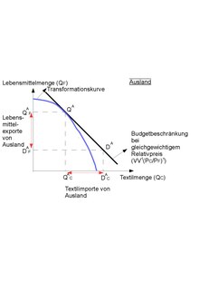
The following is a fictitious example based on Thailand and Australia. The starting point is the budget constraints of both countries and the assumption that only these two countries trade with each other . If a good is to be imported or exported, this is done automatically with the other country. At equilibrium prices, there are certain production quantities and consumption possibilities for both countries. First of all, the background: In Thailand, for example, a growth in the relative prices of one good (industrial products) leads to a growth in the consumption of the other good (food). This happens in relation to the consumption of industrial products. However, there is still a decrease in the relative production of the food. As a result of this decrease, Thailand produces less food than it consumes itself. As a result, more food is needed in the country than originally available. Thus the country imports the corresponding difference in food and becomes an exporter of industrial goods. These are imported from Australia, as trade is only carried out with this country .
Now a look at Australia: The relative price of manufactured goods is falling, bringing with it an increase in the consumption of manufactured goods relative to food. It also leads to a reduction in the relative production of industrial goods. Here, too, the situation arises that more industrial goods are required than it produces itself. At the same time, there is more food in the country than is consumed. As a result of this situation in both countries, Australia imports industrial goods and exports food. Since only these two countries trade with each other , they export and import each other.
In a state of equilibrium, the exports of one country are therefore just as large as the imports of the other. Australia therefore imports exactly the same amount of manufactured goods that Thailand exports. Thailand, in turn, imports the amount of food that Australia exports. This condition is called trade equilibrium.
Real terms of trade
definition
The Terms of Trade provide information about the quota of import goods a country can receive in the trade in export goods. Specified in its own currency.
The concepts of the terms of trade
The terms of trade are understood as real exchange relationships of goods and services between individual economies . The "Terms of Trade" can best be broken down into 3 concepts to illustrate. The Commodity Terms of Trade , Income Terms of Trade and the Factoral Terms of Trade . The requirements for the Commodity Terms of Trade are a pure exchange of goods and the existence of only one export and one import good. They are set in the ratio of the import quantity to the export quantity of a good. It is specified in which period the units of measure mix from the export to the imported goods.
The Income Terms of Trade offer an alternative to measuring welfare . Here, the export volume index and the export goods price index are set in relation to the import goods price index. In short, the commodity terms of trade are multiplied by the export volume index. This relationship makes it clear whether a country receives more or fewer units of an imported good. The Factoral Terms of Trade takes into account the effects of changes in productivity on the welfare of the respective country. Using the example of the 'labor' factor, the export price index is multiplied by the marginal productivity of the 'labor' factor and then set in relation to the import price index. In short, the commodity terms of trade are multiplied by the marginal productivity of the labor factor. Maximizing the Factoral Terms of Trade means expanding income from international trade.
Relationship between the exchange equilibrium and the terms of trade
In this context, the optimal tariff plays a corresponding role. Under normal circumstances, customs produce not only price but also volume effects. This equilibrium of exchange shows that maximizing the domestic terms of trade inevitably goes hand in hand with a minimization of domestic export volumes. If the tariff burden of the terms of trade is correspondingly high, the improvement can be so great that a cross-border exchange is no longer an option. The disadvantage associated with this is the creation of a self-sufficiency situation from the respective home and abroad. This in turn means a lower level of welfare than with foreign trade.
Exchange equilibrium
Since the trade equilibrium, as already described in the definition, represents an interstate exchange equilibrium between two countries, it will be discussed in more detail below. The term exchange is generally a voluntary act and therefore an agreement between the exchange partners about the exchange act must exist. In the case of rational individuals, for example, an exchange is possible as long as one exchange partner can improve without the other deteriorating.
Thus there is an exchange equilibrium , which represents a special form of market equilibrium and in which no production takes place if there is no further act of exchange of goods, which in this kind of equilibrium represents the only economic activity.
The quotients of the marginal rates of substitution between the exchanged goods are the same for all economic entities involved. The exchange process is shown graphically in an Edgeworth box , with the "exchange equilibrium representing those parts of the contract curve that can be reached from the initial inventory of goods."
Marginal rate of substitution
The marginal rate of substitution represents the relationship between two goods that are perceived as exchangeable by the household. It provides information about the extent to which a household is willing to forego a certain unit of quantity of one good and to receive a certain unit of quantity of the other good.
The yardstick which represents the task of one good in order to maintain the other good is thus the marginal rate of substitution.
Graphic representation

The indifference curve is rising and indicates the marginal substitute rate (MRS) of a household. The MRS of clothing by food is the amount of clothing that a household is willing to have replaced by one more unit of food. Based on the graphic, it can be concluded that the household is ready to receive one more unit of food and at the same time to forego six units of clothing (point A to B). In points B to C, the household is only willing to give up four units of clothing in order to receive an additional unit of food. Here both points are lower on the indifference curve and the household consequently has fewer units of both goods available as a whole.
Edgeworth box

"The Edgeworth Box is an analytical aid for determining the contract curve used in welfare economics, which is created by combining the indifference curve systems of two exchange partners."
Indifference curves
The indifference curves , the curvature of which depends on the functional interchangeability of certain goods, are analytical instruments of household theory and, in a two-goods model, represent all combinations of shopping baskets that allow the household the same level of utility and the two goods as equivalent to the household be assessed. An intersection between indifference curve systems would mean that they are not free of contradictions, as this implies different levels of utility on the same indifference curve.
Graphic representation
An Edgeworth box is graphically created by rotating the indifference system of B by 180 ° and placing it on top of that of A, i.e. forming a rectangle. The edge lengths correspond to the available factor or goods inventory and within these edges the indifference curves intersect or touch each other. The tangent points, connected to one another, form the contract curve.
Contract curve
The contract curve, also called negotiation, conflict, efficiency or Pareto curve, is, in simple terms, a connecting line of all exchange equilibria and thus a series of Pareto-optimal points, which say that a good cannot be placed higher without it being at the expense of the good for others.
Graphic representation
The contract curve is created within the Edgeworth box by the fact that the indifference curves of the exchange partners touch each other. It shows all Pareto-optimal situations in the Edgeworth box.
The realization of the points on the contract curve depends on the distribution of ownership in the initial situation and the negotiating skills of the exchange partners. If the point has arisen through negotiations, it must be adhered to under Pareto-optimal conditions, i.e. allocation optimal. In the tangential points, the ratios of the marginal utility of the considered goods of both exchange partners agree and are equal to the relative goods prices.
Current
The trade balance is not just a theoretical construct, it is a topical issue. It also plays a major role in an international context and is continuously discussed. For example, Federal Minister Sigmar Gabriel took up the issue in 2010 in the Handelsblatt as follows: “It would be better to orientate yourself in the European context to Karl Schiller and his“ magic square ”: price stability, combined with economic growth, high employment levels and balance in foreign trade. Because it is obvious that to overcome the current crisis of the euro, much more has to be done than just moderation in government spending. ”At this point in time, some European countries were in financial difficulties. When looking at Germany, however, it became apparent that it had far more debts than the countries concerned with economic problems. He therefore warns: “The national parliaments and governments of Europe must commit to common goals: the gradual convergence of living conditions, with the highest possible level of employment, steady economic growth, price stability, external balance and ecological sustainability. Only then does a common currency make sense. "
literature
Introductory general textbooks
- Clemens Büter: Foreign trade: Basics of global and intra-community trade relations. 2nd Edition. Springer-Verlag, Berlin / Heidelberg 2010.
- Horst Siebert: Foreign trade. 7th edition. Lucius & Lucius, Stuttgart 2000.
- Paul R. Krugman , Maurice Obstfeld : International Economy: Theory and Politics of Foreign Trade. 9th, updated edition. ISBN 978-3868941340 . Pearson, Munich 2009.
- Klaus Rose , Karlhans Sauernheimer: Theory of foreign trade. 14th edition. Vahlen Publishing House, Munich 2006.
- Gustav Dieckheuer: International economic relations. 5th edition Oldenbourg, Munich 2001.
- Gerhard Rübel : Basics of real foreign trade. Oldenbourg, Munich 2004; 2nd edition 2008.
- Borchert, Manfred: Foreign trade. Theory and politics. Springer-Verlag, 2013.
Special specialist literature
- Koska, Onur A. and Frank Stähler: Trade and imperfect competition in general equilibrium. In: Journal of International Economics 94.1 (2014), pp. 157–168.
- Green, Jerry R. and José Alexandre Scheinkman (Eds.): General equilibrium, growth, and trade. Essays in honor of Lionel McKenzie. Academic Press, 2014.
- Meade, James E.: A Geometry of International Trade (Routledge Revivals). Routledge, 2013.
- Arnold, Lutz G .: Existence of equilibrium in the Helpman-Krugman model of international trade with imperfect competition. In: Economic Theory 52.1 (2013), pp. 237–270.
- Neary, J. Peter and Joe Tharakan: International trade with endogenous mode of competition in general equilibrium. In: Journal of International Economics 86.1 (2012), pp. 118–132.
- Martimort, David and Thierry Verdier: Optimal domestic regulation under asymmetric information and international trade. A simple general equilibrium approach. In: The RAND Journal of Economics 43.4 (2012), pp. 650–677.
- Chipman, John S .: General Equilibrium and Welfare in International Trade. In: OEconomia 2012.01 (2012), pp. 15–33.
- Franke, Jan: A two-country / two-goods model without production. In: New Macroeconomics and Foreign Trade. Springer, Berlin Heidelberg, 1989, pp. 92-113.
- De Melo, Jaime and Sherman Robinson: Product differentiation and the treatment of foreign trade in computable general equilibrium models of small economies. In: Journal of international economics 27.1 (1989), pp. 47-67.
- De Melo, Jaime: Computable general equilibrium models for trade policy analysis in developing countries. A survey. In: Journal of Policy Modeling 10.4 (1989), pp. 469-503.
- Shoven, John B. and John Whalley: Applied general-equilibrium models of taxation and international trade. An introduction and survey. In: Journal of Economic Literature (1984), pp. 1007-1051.
- Bergstrand, Jeffrey H .: The gravity equation in international trade. Some microeconomic foundations and empirical evidence. In: The review of economics and statistics (1985), pp. 474-481.
- Findlay, Ronald and Henryk Kierzkowski: International trade and human capital. A simple general equilibrium model. In: The Journal of Political Economy (1983), pp. 957-978.
- Dixit, Avinash and Victor Norman: Theory of international trade. A dual, general equilibrium approach. Cambridge University Press, 1980.
Individual evidence
- ^ Paul R. Krugman, Maurice Obstfeld: International economy: theory and politics of foreign trade. 8th, updated edition. Pearson, Munich 2009, p. 154.
- ^ Paul R. Krugman, Maurice Obstfeld: International economy: theory and politics of foreign trade. 8th, updated edition. Pearson, Munich 2009, p. 134.
- ^ Paul R. Krugman, Maurice Obstfeld: International economy: theory and politics of foreign trade. 9th, updated edition. Pearson, Munich 2012, pp. 171–190
- ^ Paul R. Krugman, Maurice Obstfeld: International economy: theory and politics of foreign trade. 6th, updated edition. Pearson, Munich 2003, p. 88 ff.
- ^ Rübel, Fundamentals of real foreign trade, pp. 106-107
- ↑ Dieck Heuer, International Economics, 5th edition, p 168
- ↑ Springer Gabler Verlag (editor), Gabler Wirtschaftslexikon, keyword: Exchange equilibrium, accessed on June 10, 2015
- ↑ Springer Gabler Verlag (editor), Gabler Wirtschaftslexikon, keyword: Edgeworth-Box accessed on June 10, 2015
- ↑ Springer Gabler Verlag (editor), Gabler Wirtschaftslexikon, keyword: contract curve accessed on June 10, 2015
- ↑ a b c Sigmar Gabriel - Europe needs more than one rescue package, accessed on June 10, 2015