Cassini curve

Cassini curves with a <c a = c a> c
      

The Cassini curve (named after Giovanni Domenico Cassini ) is the location of all points in the plane for which the product of their distances from two given points and is equal . Giovanni Domenico Cassini proposed these curves as planetary orbits even after the discovery of Kepler's laws . A special case of the Cassini curve is Bernoulli's lemniscate . ${\displaystyle P_{1}}$ ${\displaystyle P_{2}}$ ${\displaystyle a^{2},a\in \mathbb {R} _{0}^{+}}$

One should not confuse the definition of a Cassini curve with the definition of an ellipse : in an ellipse the sum of the distances is constant.

Equations

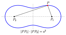
Cassini curve: definition

The curve can be expressed in Cartesian coordinates by the equation

${\displaystyle (x^{2}+y^{2})^{2}-2c^{2}(x^{2}-y^{2})=a^{4}-c^{4}\qquad a,c\in \mathbb {R} _{0}^{+}}$

describe where and was set. In polar coordinates , the equation is ${\displaystyle P_{1}=(c,0)}$ ${\displaystyle P_{2}=(-c,0)}$

${\displaystyle r^{2}=c^{2}\cos(2\varphi )\pm {\sqrt {c^{4}\cos ^{2}(2\varphi )+(a^{4}-c^{4})}}\qquad a,c\in \mathbb {R} _{0}^{+}.}$

Derivation from the definition

The problem is treated in a right-angled Cartesian coordinate system of the plane, so that and , with holds. Then, according to the definition , for a point on the curve: ${\displaystyle P_{1}=P(c,0)}$ ${\displaystyle P_{2}=(-c,0)}$ ${\displaystyle c\in \mathbb {R} _{0}^{+}}$ ${\displaystyle P=(x,y)}$

${\displaystyle {\begin{array}{rcl}a^{2}&=&|PP_{1}|\cdot |PP_{2}|={\sqrt {(x+c)^{2}+y^{2}}}{\sqrt {(x-c)^{2}+y^{2}}}\\a^{4}&=&[(x+c)^{2}+y^{2}][(x-c)^{2}+y^{2}]=(x^{2}-c^{2})^{2}+y^{2}[(x+c)^{2}+(x-c)^{2}]+y^{4}\\&=&(x^{4}-2x^{2}c^{2}+c^{4})+y^{2}[2x^{2}+2c^{2}]+y^{4}=x^{4}+2x^{2}y^{2}+y^{4}+c^{4}-2c^{2}x^{2}+2c^{2}y^{2}\\a^{4}-c^{4}&=&(x^{2}+y^{2})^{2}-2c^{2}(x^{2}-y^{2}).\end{array}}}$

The transformation is necessary for the transition to polar coordinates . It results with the " trigonometric Pythagoras ": ${\displaystyle x=r\cos(\varphi ),y=r\sin(\varphi )}$

${\displaystyle a^{4}-c^{4}=r^{4}-2c^{2}r^{2}(\cos ^{2}(\varphi )-\sin ^{2}(\varphi ))=r^{4}-2c^{2}r^{2}\cos(2\varphi ).}$

This is a quartic equation , especially the biquadratic special case, which is to be solved as a quadratic equation in : ${\displaystyle r^{2}}$

${\displaystyle (r^{2})^{2}-2c^{2}\cos(2\varphi )\cdot r^{2}-(a^{4}-c^{4})=0}$

${\displaystyle \Rightarrow r^{2}(\varphi )=c^{2}\cos(2\varphi )\pm {\sqrt {c^{4}\cos ^{2}(2\varphi )+(a^{4}-c^{4})}}.}$

Shape of the curve

The Cassini curves for different b = a / c:

b  = 0.6	b  = 0.8	b  = 1
b  = 1.2	b  = 1.4	b  = 1.6

The shape of the Cassini curve can be divided into five cases:

1st case

For the curve is an approximately elliptical oval. In this case , their points of intersection with the x-axis are enclosed , the points of intersection with the y-axis are enclosed . ${\displaystyle a>c{\sqrt {2}}}$ ${\displaystyle (\pm {\sqrt {a^{2}+c^{2}}},\,0)}$ ${\displaystyle (0,\pm {\sqrt {a^{2}-c^{2}}})}$

2nd case

For it again results in an approximately elliptical oval. The intersections with the x-axis are now included . At the intersection with the y-axis at , the curvature of the curve is equal to 0. ${\displaystyle a=c{\sqrt {2}}}$ ${\displaystyle (\pm c{\sqrt {3}},\,0)}$ ${\displaystyle (0,\,\pm c)}$

3. Case

For there is an indented oval with the same axis sections as in the case . In addition to the two y-axis segments , the other extremes of the curve are at the points ${\displaystyle c<a<c{\sqrt {2}}}$ ${\displaystyle a>c{\sqrt {2}}}$

${\displaystyle {\frac {1}{2c}}\left(\pm {\sqrt {4c^{4}-a^{4}}},\ \pm a^{2}\right)}$

The four turning points are included

${\displaystyle \left(\pm {\sqrt {{\tfrac {1}{2}}(m-n)}},\,\pm {\sqrt {{\tfrac {1}{2}}(m+n)}}\right)\quad {\text{mit}}\quad m={\sqrt {\tfrac {a^{4}-c^{4}}{3}}}\quad {\text{und}}\quad n={\tfrac {a^{4}-c^{4}}{3c^{2}}}}$

4th case

The lemniscate results for . ${\displaystyle a=c}$

5th case

For there are two ovals around the points and . The points of intersection with the x-axis have the x-coordinates ${\displaystyle a<c}$ ${\displaystyle (c,0)}$ ${\displaystyle (-c,0)}$

${\displaystyle \pm {\sqrt {c^{2}\pm a^{2}}}}$

The extremes are at the points

${\displaystyle {\frac {1}{2c}}\left(\pm {\sqrt {4c^{4}-a^{4}}},\ \pm a^{2}\right)}$

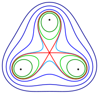
Cassini curves and orthogonal trajectories

Cassini curves and orthogonal hyperbolas

Orthogonal trajectories of a given family of curves are curves which orthogonally intersectall given curves. So are z. B. for a family of confocal ellipses the associated confocal hyperbolas orthogonal trajectories. The following applies to Cassini curves:

• The orthogonal trajectories of the Cassinian curves to two points are the equilateral hyperbolas through with the center of as the center (see picture). ${\displaystyle P_{1},P_{2}}$ ${\displaystyle P_{1},P_{2}}$ ${\displaystyle P_{1},P_{2}}$

Proof:
To make the calculation simple, be . ${\displaystyle P_{1}=(1,0),\;P_{2}=(-1,0)}$

The Cassini curves satisfy the equation

${\displaystyle f(x,y)\;=\;(x^{2}+y^{2})^{2}-2(x^{2}-y^{2})+1-a^{4}=0}$.

The equilateral hyperbolas (i.e. their asymptotes are perpendicular to each other) through and midpoint satisfy the equation ${\displaystyle (1,0),(-1,0)}$ ${\displaystyle (0,0)}$

${\displaystyle y^{2}-x^{2}+\lambda xy+1=0,\quad \lambda \in \mathbb {R} .}$

The hyperbolas do not intersect the y-axis and the x-axis only in . A major axis transformation shows that these are actually equilateral hyperbolas with the origin as the center. With point samples one recognizes: lie on the hyperbolas. In order to obtain a normal of the hyperbola that is independent of the parameter, it is better to use the following implicit representation: ${\displaystyle (\pm 1,0)}$ ${\displaystyle (1,0),(-1,0)}$

${\displaystyle g(x,y)\;=\;{\frac {x^{2}-y^{2}-1}{xy}}-\lambda ={\frac {x}{y}}-{\frac {y}{x}}-{\frac {1}{xy}}-\lambda =0\;.}$

To prove that the hyperbolas and the Cassini curves intersect perpendicularly, one shows that is for all points . This is easy to understand computationally, since the two array parameters drop out when differentiating. ${\displaystyle \operatorname {grad} f(x,y)\cdot \operatorname {grad} g(x,y)=0}$ ${\displaystyle (x,y),\;x\neq 0\neq y}$

Note:
The image of the Cassini curves and the hyperbolas orthogonal to them is similar but not the same as the field and potential lines of two identical point charges . In an equipotential line of two point charges is the sum of the reciprocals of the distances to two fixed points constant: . (See implicit curves ) ${\displaystyle {\frac {1}{|PP_{1}|}}+{\frac {1}{|PP_{2}|}}={\text{konstant}}}$

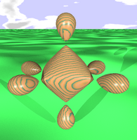
Cassini curves on Tori

Cassini curves as plane sections of a torus
(the right torus is a spindle torus )

Cassini curves also appear as plane cuts from tori . But only if the

• intersecting plane parallel to the torus axis and the distance from the torus axis is equal to the radius of the generating circle (see picture).

If you cut the torus with the equation

${\displaystyle \left(x^{2}+y^{2}+z^{2}+R^{2}-r^{2}\right)^{2}=4R^{2}\left(x^{2}+y^{2}\right).}$

with the plane we first get: ${\displaystyle y=r}$

${\displaystyle \left(x^{2}+z^{2}+R^{2}\right)^{2}=4R^{2}\left(x^{2}+r^{2}\right).}$

After partially resolving the first bracket, the result is

${\displaystyle \left(x^{2}+z^{2}\right)^{2}-2R^{2}(x^{2}-z^{2})=4R^{2}r^{2}-R^{4}.}$

The and coordinates of the intersection curve satisfy the equation of a Cassini curve with the parameters . ${\displaystyle x}$ ${\displaystyle z}$ ${\displaystyle a^{2}=2Rr,\;c=R}$

For further torus cuts: see Villarceau circles , spiral curve .

Generalizations

The construction of a Cassini curve can easily be generalized to flat curves and surfaces with any number of basic points:

• ${\displaystyle |PP_{1}|\cdot |PP_{2}|\cdots |PP_{n}|=a^{n}}$

describes an implicit curve in the plane case and an implicit surface in the 3-dimensional space .

• 

  general 3 point curves

• 

  general Area to 6 points

literature

• Bronstein among other things: Pocket book of mathematics . Publisher Harri Deutsch, Frankfurt am Main 2005, ISBN 3-8171-2006-0 .

• I. Agricola, T. Friedrich: Elementarge Geometry: Expertise for Studies and Mathematics Lessons , Springer Spectrum, 2015, ISBN 978-3-658-06730-4 , p. 60.

Web links

• Weisstein, Eric W. "Cassini Ovals." From MathWorld - A Wolfram Web Resource.
• 2Dcurves.com description is not working
• "Ovale de Cassini" at Encyclopédie des Formes Mathématiques Remarquables (in French)