Utility function (microeconomics)

In economics and especially in microeconomics, a utility function is a mathematical function that describes the preferences of economic subjects . It assigns a real number to any bundle of goods , in such a way that more highly valued bundles of goods receive larger numbers. The assigned numbers are called benefits of the respective bundle of goods.

In microeconomic theory, utility functions only contain statements about the hierarchy: If one bundle of goods delivers a higher utility than another, it can only be concluded that the former is “better” than the latter from the point of view of the economic subject concerned; how big the distance between the numbers is has no meaning. Such utility functions are also called ordinal utility functions, because they merely specify an order of the bundle of goods. The concept of the ordinal utility function is based on a different theoretical foundation than the so-called cardinal utility functions, in which the difference between the utility value of two goods can also be interpreted.

The concept of the utility function is used both directly in microeconomics and in the context of macroeconomic issues.

The goal of maximizing utility is often accepted as the action-determining striving of the consumer (cf. Homo oeconomicus ). An alternative goal would be satisficing (a requirement fulfillment ).

definition

In the following, it is assumed that the utility can only be measured ordinally, and the utility function is introduced as it is constructed in household theory .

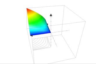
Illustrative definition in the two-goods case

Utility function in the two-goods case (here: Cobb-Douglas utility function, see below).
${\displaystyle u(x_{1},x_{2})={\sqrt {x_{1}}}\cdot {\sqrt {x_{2}}}}$

If one restricts the scope of the bundle of goods to two goods for the sake of simplicity, one can, for example, imagine a bundle of goods A made up of two types of goods: kiwi (good 1) and cherries (good 2). Goods bundle A now contains a certain amount of kiwi - marked with - and a certain amount of cherries - marked with ; one writes short for this bundle of goods . Similarly, imagine a second bundle of goods B made of kiwi and cherries, which is represented accordingly by . With concrete values, one can imagine, for example, that goods bundle A contains two kiwi and six cherries while . If one assumes, as usual, that the preferences are monotonous (casually: “more is better”), household should prefer B to A. There are an infinite number of utility functions that can map the preferences, since all they have to do is ensure that the function value at that point is greater than that at that point . For example, to read a function used with the and . Negative values ​​are also possible: If there is a different utility function and / or , then this utility function is also consistent with the preferences of the household. ${\displaystyle x_{1}^{A}}$ ${\displaystyle x_{2}^{A}}$ ${\displaystyle A=(x_{1}^{A},x_{2}^{A})}$ ${\displaystyle B=(x_{1}^{B},x_{2}^{B})}$ ${\displaystyle A=(2,6)}$ ${\displaystyle B=(3,6)}$ ${\displaystyle (3,6)}$ ${\displaystyle (2,6)}$ ${\displaystyle u_{1}}$ ${\displaystyle u_{1}(A)=300}$ ${\displaystyle u_{1}(B)=890}$ ${\displaystyle u_{2}}$ ${\displaystyle u_{2}(A)=-3}$ ${\displaystyle u_{2}(B)=-1}$

Similarly, combinations of goods that the household likes equally must have the same utility values. If, for example, the bundle of goods is perceived as being just as good as the bundle of goods , then that must also apply to every utility function . ${\displaystyle C=(4,10)}$ ${\displaystyle D=(2,11)}$ ${\displaystyle u(C)=u(D)}$

Formal definition

In microeconomic theory, one assumes that economic subjects have preferences about the choice alternatives that are potentially available to them. Mathematically, such preferences (which can be very general) can be represented as binary relations . For example, a preference-indifference relation is agreed in this way. Now let and be vectors of goods from a set of alternatives, then it is expressed by that the goods bundle is rated at least as good as or better than . In order to preserve this information in the corresponding utility function, the function value of the utility function for must be equal to or higher than that of . This leads to the following exact definition: ${\displaystyle R}$ ${\displaystyle \mathbf {x} _{a}}$ ${\displaystyle \mathbf {x} _{b}}$ ${\displaystyle X}$ ${\displaystyle \mathbf {x} _{a}R\mathbf {x} _{b}:=(\mathbf {x} _{a},\mathbf {x} _{b})\in R}$ ${\displaystyle \mathbf {x} _{a}}$ ${\displaystyle \mathbf {x} _{b}}$ ${\displaystyle \mathbf {x} _{a}}$ ${\displaystyle \mathbf {x} _{b}}$

Definition: A function is a utility function that indifference-preference ratio which reflects when all bundle of goods applies: . ${\displaystyle u\colon X\rightarrow \mathbb {R} }$ ${\displaystyle R}$ ${\displaystyle \mathbf {x} _{a},\mathbf {x} _{b}\in X}$ ${\displaystyle \mathbf {x} _{a}R\mathbf {x} _{b}\Leftrightarrow u(\mathbf {x} _{a})\geq u(\mathbf {x} _{b})}$

Utility functions make it possible to represent certain preference-indifference relations in an equivalent functional manner (see also the section Existence of a utility function in this article). Their advantage lies in their comparatively much simpler mathematical manageability.

As with the analysis of the preference relations, indifference and strict preference can be derived from the preference-indifference relation. The definition of strict preference is: For two alternatives and is if and only if (1) but (2) not at the same time . If we are dealing with a utility function, the above definition applies because of (1) that and because of (2) that not , which just implies, that with strict preference actually applies . Similarly, it can also be seen for the indifference relation that, according to the above definition of , it is expressed in the utility function precisely by the fact that for two bundles of goods considered to be equivalent . How large the distance between the function values ​​is or how high the function values ​​themselves are is irrelevant. ${\displaystyle P}$ ${\displaystyle \mathbf {x} _{a}}$ ${\displaystyle \mathbf {x} _{b}}$ ${\displaystyle \mathbf {x} _{a}P\mathbf {x} _{b}}$ ${\displaystyle \mathbf {x} _{a}R\mathbf {x} _{b}}$ ${\displaystyle \mathbf {x} _{b}R\mathbf {x} _{a}}$ ${\displaystyle u}$ ${\displaystyle u(\mathbf {x} _{a})\geq u(\mathbf {x} _{b})}$ ${\displaystyle u(\mathbf {x} _{b})\geq u(\mathbf {x} _{a})}$ ${\displaystyle u(\mathbf {x} _{a})>u(\mathbf {x} _{b})}$ ${\displaystyle I}$ ${\displaystyle R}$ ${\displaystyle \mathbf {x} _{a},\mathbf {x} _{b}:u(\mathbf {x} _{a})=u(\mathbf {x} _{b})}$

Classification and properties

Utility concept and transformations of the utility function

The interpretation on which the above definition is based is quite general, in such a way that the specific utility values ​​cannot be interpreted individually - when comparing bundles of goods it is only a question of how the two corresponding utility values ​​relate to one another, i.e. whether one is greater or equal or smaller than the other. This is based on the approach of considering the measurability of the benefit as exclusively ordinal . The utility concept of modern household theory is based on this assumption, since the preference relations do not contain any further information (pairwise comparison of alternatives). It is so intuitively understood that utility functions in the sense defined above can positively strictly be transformed monotonous and arbitrary, so that the same information contains as if only strictly increasing in is. ${\displaystyle f\left[u(\mathbf {x} )\right]}$ ${\displaystyle u(\mathbf {x} )}$ ${\displaystyle f\colon \mathbb {R} \rightarrow \mathbb {R} }$ ${\displaystyle u}$

Other types of utility functions are also conceivable - but not compatible with the above concept. For example , if the utility is measured on a cardinal scale , a transformation would only be permissible if it is positive affine, i.e. if . The more restrictive requirements of the cardinal scale, however, correspond with expanded interpretation possibilities, because here it would be quite possible to infer from the fact that the utility value increases by 10 when moving from bundles of goods , while it increases by 20 when moving from to , that the additional Benefit from opposite is twice as high as that from opposite . ${\displaystyle f}$ ${\displaystyle f\left[u(\mathbf {x} )\right]=a+b\cdot u,\;b>0}$ ${\displaystyle \mathbf {x} _{a}}$ ${\displaystyle \mathbf {x} _{b}}$ ${\displaystyle \mathbf {x} _{a}}$ ${\displaystyle \mathbf {x} _{c}}$ ${\displaystyle \mathbf {x} _{c}}$ ${\displaystyle \mathbf {x} _{a}}$ ${\displaystyle \mathbf {x} _{b}}$ ${\displaystyle \mathbf {x} _{a}}$

If the utility is measured on a ratio scale , a transformation would only be permissible if it is positive linear, i.e. if . Here one could conclude from the fact that the benefit of bundles of goods is twice as great as that of , that the former bundle also provides twice as high a benefit as the latter. ${\displaystyle f}$ ${\displaystyle f\left[u(\mathbf {x} )\right]=b\cdot u,\;b>0}$ ${\displaystyle \mathbf {x} _{a}}$ ${\displaystyle \mathbf {x} _{b}}$

In the extreme case, no transformation at all is permitted ( absolute scale ) , in which case even the absolute level of benefit (for example ) could be interpreted. ${\displaystyle u(\mathbf {x} _{a})=12}$

Existence of a utility function

If one assumes the existence of a preference order, this cannot be represented in all cases by a utility function. Rather, additional requirements must be placed on the quantity of alternatives or the order of preferences.

→ Main article : Preference relation

Functional properties

Based on the associated orders of preference, statements can also be made about the properties of a utility function.

Relationship between the properties of the preference relation and the properties of the utility function constructed from it:

• ${\displaystyle u(\mathbf {x} )}$is strictly monotonically increasing if and only if the underlying preference-indifference relation fulfills the property of strict monotonicity. ${\displaystyle R}$
• ${\displaystyle u(\mathbf {x} )}$is quasi-concave if and only if the underlying preference-indifference relation is convex. ${\displaystyle R}$
• ${\displaystyle u(\mathbf {x} )}$is even strictly quasi-concave if and only if the underlying preference-indifference relation is strictly convex. ${\displaystyle R}$

A preference-indifference relation is called strictly monotonic if ; as convex if and as strictly convex if . See the article Preference Relation in more detail . ${\displaystyle \forall \mathbf {x} _{a},\mathbf {x} _{b}:(\mathbf {x} _{a}\geq \mathbf {x} _{b})\wedge (\mathbf {x} _{a}\neq \mathbf {x} _{b})\implies \mathbf {x} _{a}P\mathbf {x} _{b}}$ ${\displaystyle \forall \mathbf {x} _{a},\mathbf {x} _{b},\mathbf {x} _{c}:\mathbf {x} _{a}R\mathbf {x} _{c}\wedge \mathbf {x} _{b}R\mathbf {x} _{c}\implies \forall t\in [0,1]:(t\mathbf {x} _{a}+(1-t)\mathbf {x} _{b})R\mathbf {x} _{c}}$ ${\displaystyle \forall \mathbf {x} _{a},\mathbf {x} _{b},\mathbf {x} _{c}:(\mathbf {x} _{a}R\mathbf {x} _{c}\wedge \mathbf {x} _{b}R\mathbf {x} _{c})\wedge (\mathbf {x} _{a}\neq \mathbf {x} _{b})\implies \forall t\in (0,1):(t\mathbf {x} _{a}+(1-t)\mathbf {x} _{b})P\mathbf {x} _{c}}$

Indifference curve

Three indifference curves in the two-goods case.

Indifference curves in the three-goods case

→ Main article : Indifference curve

As defined above, utility functions indicate the utility level that certain bundles of goods generate. If you look at the function from a different angle, you can also specify a certain level of benefit and ask about the bundles of goods with which this can be achieved. This forms the basis for the concept of an indifference curve (also utility isoquant or iso utility function ). If one assumes a bundle of goods , then an indifference curve is formally the set of all bundles of goods for which (indifference amount to ) applies . ${\displaystyle {\overline {u}}}$ ${\displaystyle \mathbf {x} _{a}}$ ${\displaystyle \mathbf {x} }$ ${\displaystyle \mathbf {x} I\mathbf {x} _{a}}$ ${\displaystyle \mathbf {x} _{a}}$

In the two-goods case, indifference curves can be visualized quite easily as shown opposite. Between the horizontal and the vertical axis is the amount of all possible bundles of goods (each point in this area marks a certain combination of good 1 and good 2). On the indifference curve 2, for example, there are all points that bring the household the same benefit as B and you can see, among other things, that the household is indifferent between C and B (that is, C and B are equally good). If, as usual, one assumes that the preferences are monotonous (“more is better”), indifference curves stand for a higher level of utility the further they are from the origin - the bundles of goods on indifference curve 2 are therefore always better than those on curve 1.

Mathematically, an indifference set in the sense defined above is a level set for the utility function. For example, if a utility function, then include the bundle of goods , and points to the indifference curve for utility level 4, because . ${\displaystyle u(x_{1},x_{2})={\sqrt {x_{1}x_{2}}}}$ ${\displaystyle (2,8)}$ ${\displaystyle (8,2)}$ ${\displaystyle (4,4)}$ ${\displaystyle u(2,8)=u(8,2)=u(4,4)={\overline {u}}={\sqrt {16}}}$

Visualization of the property as a level set - indifference curves as contour lines of the utility function. In the example: Cobb-Douglas utility function as above; Four contour lines / indifference curves are drawn in the (x1, x2) plane. (Note that the x2 axis here for clarity x1 axis do not intersect at the zero point, one imagines the axis on the other hand to the left front, the familiar image shows an indifference curve in the two-goods case.)

Play media file

“Projection” of the contour lines in the x1-x2 plane (animation).

It also follows from this property that indifference curves cannot intersect. If A and B were two genuinely different sets of indifference and if there were a bundle of goods that are contained in both A and B , then this would necessarily lead to a contradiction. According to the definition of an indifference set, it would apply to all other bundles of goods from A that they generate the same utility as (because it is contained in A); for all other bundles of goods from B the same applies (because it is contained in B), which means that all bundles of goods in A and B generate the same benefit as . Then the indifference sets cannot really be different - contrary to the assumption. ${\displaystyle \mathbf {x} '}$ ${\displaystyle \mathbf {x} '}$ ${\displaystyle \mathbf {x} '}$ ${\displaystyle \mathbf {x} '}$ ${\displaystyle \mathbf {x} '}$

Marginal utility and marginal rate of substitution

Marginal utility

→ Main article : marginal utility

The first partial derivation of the utility function for a good is called the marginal utility of this good. The marginal utility clearly indicates how much additional utility a marginal increase in the amount of goods would generate, with the amount of all other goods being left unchanged. A marginal utility of means that this good is saturated. A further unit of this good (with a concave function curve) would provide no additional benefit. ${\displaystyle \partial u(\mathbf {x} )/\partial x_{i}}$ ${\displaystyle x_{i}}$ ${\displaystyle x_{i}}$ ${\displaystyle 0}$

It should be borne in mind that just like the utility function, the marginal utility function or the marginal utility of a good in itself has no meaningfulness. For example, if one considers a utility function in the two-goods case , then the marginal utility of good is 2 . However, a strictly monotonous positive transformation of the utility function leads to the marginal utility of good 2 now amounting to - that is, it is also tripled, which makes it clear that marginal utility values ​​can be transformed at will. However, it turns out that the relationship between the marginal utility of various goods can be interpreted very well, as the following section shows. ${\displaystyle u(x_{1},x_{2})=x_{1}+3x_{2}^{2}}$ ${\displaystyle 6x_{2}}$ ${\displaystyle v=3\cdot u(x_{1},x_{2})=3x_{1}+9x_{2}^{2}}$ ${\displaystyle 18x_{2}}$

Illustration of Gossen's First Law. The quantity of goods is plotted on the horizontal axis and the utility on the vertical axis (utility function in the case of single goods).

In some applications it is believed that the marginal utility of goods is typically decreasing in quantity; Hermann Heinrich Gossen already made the assertion within the framework of his utility theory that the additional utility of further units of a good would decrease the more units one already had of the good ( first Gossen's law ). However, it must be borne in mind that the assumption is not compatible with an ordinal utility theory as it was based on the budget theory above. This is because the utility values ​​are of no importance - the fact that a utility function with and is equivalent to with or shows that corresponding permissible modifications of the utility function can significantly influence the marginal utility change, from which it follows that the to- or diminishing character when applying an ordinal concept does not offer any interpretation. ${\displaystyle u_{1}}$ ${\displaystyle u_{1}(1,1)=1}$ ${\displaystyle u_{1}(1,2)=2}$ ${\displaystyle u_{2}}$ ${\displaystyle u_{2}(1,1)=1}$ ${\displaystyle u_{2}(1,2)=100}$

Another common assumption is a strictly positive marginal utility, i.e. every additional unit of a good generates an additional utility. In the preference theory foundation, this assumption corresponds to the assumption of strict monotony of household preferences, according to which a strictly preferred bundle of goods exists in every environment of a bundle of goods, in which there is the same amount of all remaining goods, but more of at least one good.

Marginal rate of substitution

In the two-goods case, the absolute amount of the slope of an indifference curve is also called the marginal rate of substitution . It is ${\displaystyle (GRS)}$

${\displaystyle {\mathit {GRS}}_{1,2}(x_{1},x_{2})\equiv |f'(x_{1})|=-f'(x_{1})={\frac {\partial u(x_{1},x_{2})/\partial x_{1}}{\partial u(x_{1},x_{2})/\partial x_{2}}}}$

(read: marginal rate of substitution of good 1 with respect to good 2), i.e. precisely the ratio of marginal utility.

This can be shown as follows: Since in falls, is and thus also what the penultimate equation explains. It is also true for a bundle of goods that the indifference curve lies in the plane, so that it can be noted directly as a function for which . This means that the bundle of goods can be represented as and, according to the definition of the indifference curve, it applies that (constant). The derivation of regarding is now beyond ${\displaystyle f}$ ${\displaystyle x_{1}}$ ${\displaystyle f'(\cdot )<0}$ ${\displaystyle |f'(x_{1})|=-f'(x_{1})}$ ${\displaystyle \mathbf {x} =(x_{1},x_{2})}$ ${\displaystyle (x_{1},x_{2})}$ ${\displaystyle x_{2}=f(x_{1})}$ ${\displaystyle (x_{1},f(x_{1}))}$ ${\displaystyle u(x_{1},f(x_{1}))={\overline {u}}}$ ${\displaystyle u(\cdot )}$ ${\displaystyle x_{1}}$

${\displaystyle {\frac {\partial u(x_{1},x_{2})}{\partial x_{1}}}+{\frac {\partial u(x_{1},x_{2})}{\partial x_{2}}}f'(x_{1})=0}$

(it corresponds because of ), which together with exactly leads to the listed equation of the GRS - which was to be shown. ${\displaystyle 0}$ ${\displaystyle {\overline {u}}=\mathrm {const.} }$ ${\displaystyle {\mathit {GRS}}=-f'(x_{1})}$

The GRS indicates the exchange ratio with which a household is willing to exchange a marginal unit of good 2 for one of good 1. This marginal rate of substitution is invariant to positive, strictly monotonic transformation. The concept can also be used for a larger number of goods, in which case for any goods : ${\displaystyle a,b}$

${\displaystyle {\mathit {GRS}}_{a,b}(\mathbf {x} )={\frac {\partial u(\mathbf {x} )/\partial x_{a}}{\partial u(\mathbf {x} )/\partial x_{b}}}}$.

The MRS is usually assumed to fall strictly monotonically, which is equivalent to the statement that indifference curves are convex and also corresponds directly to the convexity assumption of the preferences in the preference-theoretical foundation. Intuitively, in the two-goods case, this means that if you do not have a marginal unit of good 2, you have to be compensated with more units of good 1, the less you have of good 2.

See also : marginal social utility  and substitute good

Examples of utility functions

Cobb-Douglas and CES utility function

→ Main articles : Cobb-Douglas function  and CES function

A Cobb-Douglas utility function is usually a utility function of the form

${\displaystyle u(\mathbf {x} )=\beta \cdot \prod _{i=1}^{n}x_{i}^{\alpha _{i}}=\beta \cdot x_{1}^{\alpha _{1}}\cdot \dotsc \cdot x_{n}^{\alpha _{n}}}$

with ; and for everyone . In simplified terms, however, in the two-goods case one often makes the assumption that and that the exponents just add up to one, which ensures constant returns to scale : ${\displaystyle \beta >0}$ ${\displaystyle x_{i}>0}$ ${\displaystyle \alpha _{i}>0}$ ${\displaystyle i=1,\dotsc ,n}$ ${\displaystyle \beta =1}$

${\displaystyle u(x_{1},x_{2})=x_{1}^{\alpha }\cdot x_{2}^{1-\alpha }}$with . ${\displaystyle \alpha \in (0,1)}$

The Cobb-Douglas utility function is a common subclass of the general CES utility function

${\displaystyle u(\mathbf {x} )=\beta \cdot \left[\alpha _{1}x_{1}^{-\rho }+\alpha _{2}x_{2}^{-\rho }+\dotsc +\alpha _{n}x_{n}^{-\rho }\right]^{-\gamma /\rho }}$

with ; and for everyone as well . It converges for straight against the Cobb-Douglas function. ${\displaystyle \beta ,\gamma >0}$ ${\displaystyle x_{i}>0}$ ${\displaystyle \alpha _{i}>0}$ ${\displaystyle i=1,\dotsc ,n}$ ${\displaystyle \rho \neq 0}$ ${\displaystyle \rho \rightarrow 0}$

Quasi-linear utility function

→ Main article : Quasilinear utility function

A utility function is quasi-linear if it has the form , where again is a utility function. In the simplest case and is accordingly . The function is quasi-linear in , that is, it is "partially linear". In the two-goods case, indifference curves differ graphically from quasi-linear utility functions only in terms of the height of the vertical axis intercept. For a given amount of good 1, all indifference curves have the same slope. In the case of quasi-linear preferences, there is no local income effect as long as the income m is large enough, i.e. the change in demand as a result of a change in the price of any good is entirely due to the substitution effect. ${\displaystyle u(\mathbf {x} )=x_{1}+v(x_{2},\ldots ,x_{n})}$ ${\displaystyle v(\cdot )}$ ${\displaystyle \mathbf {x} =(x_{1},x_{2})}$ ${\displaystyle u(x_{1},x_{2})=x_{1}+v(x_{2})}$ ${\displaystyle x_{1}}$

Limitative utility function

→ Main article : "Limitational" in the article production function

In the case of the limiting utility function, the factors are in a specific application ratio, ie the utility only increases if both factors are increasingly used. A frequently used limited utility function is the Leontief production function .

Intertemporal utility function

An intertemporal utility function maps preferences via consumption alternatives that are available at different times. Among other things, it can be used to explain why and how much people are saving or taking out loans .

In line with empirically observable behavior, one often assumes that individuals prefer more timely consumption to more distant consumption of the same amount with intertemporal preferences; one speaks here of a positive time preference . In utility functions, this positive time preference is often represented by discount factors , whereby, for the sake of simplicity, one often assumes a constant rate of time preference even with changes in income.

For example, in overlapping generation models it is usually assumed that individuals live exactly two periods: In the first period they have an income that they can consume or save. In the second period they live on their (interest-bearing) savings and additional, smaller equipment (for example a state subsidy). The individuals then maximize utility over their entire life-cycle consumption, that is, they maximize an intertemporal utility function ${\displaystyle \omega _{t}^{1}}$

${\displaystyle U^{t}\left(c_{t}^{1},c_{t}^{2}\right)}$,

where in the sketched example, simplistic and in the absence of transfer systems and ( is the consumption of an individual born in in period , is the consumption of an individual born in in period (i.e. precisely his second phase of life), is the interest rate on the savings between period and ). ${\displaystyle c_{t}^{1}=\omega _{t}^{1}-s_{t}}$ ${\displaystyle c_{t}^{2}=\left(1+r_{t+1}\right)s_{t}+\omega _{t}^{2}}$ ${\displaystyle c_{t}^{1}}$ ${\displaystyle t}$ ${\displaystyle t}$ ${\displaystyle c_{t}^{2}}$ ${\displaystyle t}$ ${\displaystyle t+1}$ ${\displaystyle r_{t+1}}$ ${\displaystyle s_{t}}$ ${\displaystyle t}$ ${\displaystyle t+1}$

The time preference rate of an economic subject is the private time preference rate , while that of a society is referred to as the social time preference rate . The concept of the indifference curve can be applied analogously.

Von-Neumann-Morgenstern expected utility function

Microeconomically, decisions under uncertainty are often modeled as a lottery . The benefit of choosing an alternative is not immediately known here. Instead of a utility function, an expected utility function (also known as the VNM utility function ) is used to model the actor's preferences.

The expected value is defined as a utility value for the individual alternatives via a (typically one-dimensional) utility function. The utility function of the respective alternatives and their probability distribution therefore determine the utility of a lottery: Expected utility is simply the expected value of the utility of the alternatives. Such a utility function is also referred to as a Von-Neumann - Morgenstern (expectation) utility function.

${\displaystyle V(z)=\operatorname {E} [u(z)]=\sum _{i=1}^{N}p_{i}\cdot u(z_{i})}$

${\displaystyle V}$denotes the expected utility function over the random variable ( states that occur with different probabilities ) and is the so-called Bernoulli utility function as a function of . The Von-Neumann-Morgenstern utility function is thus nothing other than the utility weighted with the probabilities from the various states that can result from the lottery. ${\displaystyle z}$ ${\displaystyle i}$ ${\displaystyle p}$ ${\displaystyle u}$ ${\displaystyle z}$

The existence of an expected utility function, however, requires stronger assumptions, in particular the controversial axiom of independence , according to which irrelevant alternatives must not have any influence on the result. Regardless of the admissibility of an expected utility formulation , economic agents can be classified as risk-averse , risk-neutral or risk-averse .

Risk aversion

Utility functions in expected utility theory differ according to the degree of risk aversion of individuals expressed in them . An individual is called risk averse if he prefers a lottery with the expected value a to have a secure income of a , for example, if the individual prefers the secure amount of 50 euros to a lottery where there is a 50 percent probability of 100 euros , but with a 50 percent probability only receives 0 euros. It can be shown that under common assumptions an individual is risk averse if and only if his Von-Neumann-Morgenstern expectation utility function is strictly concave.

According to the Arrow-Pratt measure , the utility functions result in the following subclasses:

• CRRA : Constant relative risk aversion
• IRRA : Increasing relative risk aversion
• DRRA : Decreasing relative risk aversion
• IARA : Increasing absolute risk aversion
• DARA : Decreasing absolute risk aversion
• CARA : Constant absolute risk aversion

HARA utility functions

In financial economics , a class of utility functions summarized under the term HARA (hyperbolic absolute risk aversion) is used.

The general form of the HARA utility function is

${\displaystyle u(c)={\frac {1-\gamma }{\gamma }}\left({\frac {ac}{1-\gamma }}+b\right)^{\gamma }}$

where is the level of consumption. The function must be continuously completed for the Bernoulli case ( ) and the risk-neutral case ( ) using the de l'Hospital rule . ${\displaystyle c}$ ${\displaystyle \gamma =0}$ ${\displaystyle \gamma =1}$

If and , the result is the isoelastic utility function , which is identical to the CRRA class. It is often considered in the consumer investment problem , since bankruptcy cannot appear in the model there, it is empirically relatively adequate and mathematically it is still relatively easy to handle. (Merton's seminal papers also looked at other cases, but the solutions were incorrect and included negative consumption.) The classic Bernoulli log utility function is a special case of the isoelastic utility function. It can be proven that all CRRA utility functions belong to the HARA class. ${\displaystyle a=1}$ ${\displaystyle b=0}$

The exponential utility function is also often used because of its easy analytical manageability. It has the form and arises for and . The parameter determines the risk preference here . It belongs to the CARA class. If only the risk averse cases are to be considered, i.e. H. , it can be simplified. ${\displaystyle u(c)=-\exp(-ac)/a}$ ${\displaystyle b=1}$ ${\displaystyle \lambda \to -\infty }$ ${\displaystyle a}$ ${\displaystyle a>0}$ ${\displaystyle u(c)=-\exp(-ac)}$

Indirect utility function

→ Main article : Indirect utility function

In the context of the utility maximization problem that arises when constructing Marshall's demand functions, a special “utility function” is often used, the so-called indirect utility function. It is usually designated with and is constructed in such a way that, depending on the goods prices and the household budget, it directly indicates the maximum level of benefit that would have resulted from the solution of the corresponding maximization problem under constraints. ${\displaystyle v}$

Recoverability problem

A recoverability problem is the question of determining the order of preferences from a utility function that generates the utility function presented. This is the reverse of the problem of finding a utility function with certain characteristics for an order of preference.

Macroeconomic Benefit Theory

In the macroeconomic context, macroeconomic utility functions are used to measure the advantageousness of certain political and economic developments for macroeconomic development.

In macroeconomics, the concept is also used to model the behavior of economic policy actors. In this context, for example, utility functions for re-election-oriented politicians are created within the framework of public choice theory . According to this, politicians will choose the political alternative that makes the most of their re-election opportunities.

See also

• Prospect Theory

literature

• Anton Barten and Volker Böhm: Consumer Theory. In: Kenneth J. Arrow and Michael D. Intrilligator (Eds.): Handbook of Mathematical Economics. Vol. 2. North Holland, Amsterdam 1982, ISBN 978-0-444-86127-6 , pp. 382-429.
• Geoffrey A. Jehle and Philip J. Reny: Advanced Microeconomic Theory. 3rd ed. Financial Times / Prentice Hall, Harlow 2011, ISBN 978-0-273-73191-7 .
• Andreu Mas-Colell, Michael Whinston, and Jerry Green: Microeconomic Theory. Oxford University Press, Oxford 1995, ISBN 0-195-07340-1 .
• George J. Stigler : The Development of Utility Theory. I. In: Journal of Political Economy. 58, No. 4, 1950, pp. 307-327.
• George J. Stigler: The Development of Utility Theory. II. In: Journal of Political Economy. 58, No. 5, 1950, pp. 373-396.
• Hal Varian : Intermediate Microeconomics. A modern approach. 8th edition. WW Norton, New York and London 2010, ISBN 978-0-393-93424-3 .
• Susanne Wied-Nebbeling and Helmut Schott: Fundamentals of microeconomics. Springer, Heidelberg a. a. 2007, ISBN 978-3-540-73868-8 .

Individual evidence

1. ↑ Cf. Geoffrey A. Jehle and Philip J. Reny 2011, p. 17.
2. ↑ See, for example, Mas-Colell / Whinston / Green 1995, p. 9.
3. ↑ Geoffrey A. Jehle and Philip J. Reny 2011, p. 17.
4. ↑ Geoffrey A. Jehle and Philip J. Reny 2011, p. 18.
5. ^ S. Sethi: Optimal Consumption and Investment with Bankruptcy , Kluwer (1997).