Linear progressive tariff

The linear-progressive tariff is a variant of the progressive income tax tariff in which the increasing course of the marginal tax rate between the initial and the top tax rate is linear (straight). This avoids sudden transitions between tariff zones and "tariff humps".

General example

Tax amount function (general example)

Marginal tax rate function (general example)

Average tax rate function (general example)

The following general example shows the calculation using a tariff with the following characteristics:

• Basic tax allowance: 10,000 euros
• Input tax rate: 10%
• Upper income threshold: 90,000 euros
• Top tax rate: 50%

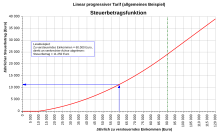
The marginal tax rate increases linearly by 0.5 percentage points for every EUR 1000 increase in income. Given is a taxable income (zvE) of 60,000 euros.

Tax amount function

As a rule, a calculation rule ( tax amount function ) is defined in the law , which provides the individual tax amount in euros as a result, if the taxable income is given.

If this relationship is shown graphically, the curve in the picture at the top right results, from which the tax amount can be read off directly. Most of the time, however, tax tables or computer programs are available that provide the tax amount you are looking for.

In the above example, the tax amount is 11,250 euros.

Marginal tax rate function

To illustrate the marginal tax burden, the trend of the marginal tax rate is often shown graphically. It is not possible to read the tax amount directly from this diagram.

The tax amount is obtained indirectly by calculating the area below the function graph , which is determined by the limits of the basic tax allowance and the individual zvE. Since it is a rectangular trapezoidal area , the tax amount can be calculated from the mean marginal tax rate and the distance between the basic tax allowance and the zvE. In the example, the average marginal tax rate is 22.5%.

${\displaystyle {\begin{aligned}{\text{Steuerbetrag}}&={\tfrac {10\ \%+35\ \%}{2}}\ \cdot \ (60\,000-10\,000){\text{ Euro}}\\&=\ \ 22{,}5\ \%\ \cdot \ 50\,000{\text{ Euro}}\\&=11\,250{\text{ Euro}}\end{aligned}}}$

Average tax rate function

The calculation of the tax amount using the average tax rate is somewhat easier . This can be easily read from the graph for the average tax rate function.

With the determined average tax rate of s = 18.75% and given zvE = 60,000 euros, the tax amount is then obtained by multiplying these two values. So in the example

${\displaystyle {\text{Steuerbetrag}}=18{,}75\ \%\cdot 60\,000{\text{ Euro}}=11\,250{\text{ Euro}}}$

Mathematical definition

The linear-progressive course of the marginal tax rate can be imagined as a result of a tiered limit rate tariff in which the number of stages is greatly increased and at the same time their level is reduced. A tax amount function is created which increases the marginal tax rate proportionally to the taxable income (zvE). A quadratic function of the form results from these specifications

${\displaystyle StB=s_{g1}\cdot (zvE-GFB)+p_{1}\cdot (zvE-GFB)^{2}}$

or ( zvE - GFB ) excluded

${\displaystyle StB={\Big (}s_{g1}+p_{1}\cdot (zvE-GFB){\Big )}\cdot (zvE-GFB)}$

This tax amount function contains the following parameters:

• ${\displaystyle StB}$ = Tax amount
• ${\displaystyle zvE}$ = taxable income
• ${\displaystyle GFB}$ = Basic allowance
• ${\displaystyle s_{g1}}$ = Initial tax rate (initial marginal tax rate)
• ${\displaystyle p_{1}}$ = linear progression factor

Since the marginal tax rate represents the slope of the tax amount function, the derivation gives : ${\displaystyle s_{g}}$

${\displaystyle s_{g}=s_{g1}+2\cdot p_{1}\cdot (zvE-GFB)}$

As you can see, it is a linear function, which explains the name. With a given marginal tax rate function, the tax amount is the other way around by integration , which can be clearly interpreted as a calculation of the area .

The following applies to the average tax rate with basic allowance: ${\displaystyle {\bar {s}}}$

${\displaystyle {\bar {s}}={\Big (}s_{g1}+p_{1}\cdot (zvE-GFB){\Big )}\cdot \left(1-{\frac {GFB}{zvE}}\right)}$

Even without a basic tax allowance ( GFB = 0), linear progression has a progressive effect because the progression factor continuously increases the average tax rate depending on the . In practice, however, a basic allowance is always provided because of the tax exemption for the subsistence level. The average tax rate for low and middle incomes is flatter than the average tax rate for a flat tax . ${\displaystyle p_{1}}$ ${\displaystyle zvE}$

Germany

Income tax tariff reform 1990 in Germany

→ Main article : Income tax (Germany)

In Germany, a linear-progressive tariff was first announced under the Helmut Kohl government in 1984. In 1990, under Finance Minister Theo Waigel, a continuously linear-progressive income tax rate came into force, which had previously been enforced by Gerhard Stoltenberg . This created a tariff course without bumps and jumps. At that time the " middle class belly " that had existed since the 1960s was eliminated.

In the following years until today this course has changed again and again. Since then, it has consisted of two or three zones with different inclines.

Individual evidence

1. ↑ ^{a b} Klaus Tipke : "An end to the income tax confusion !?", Cologne 2006, page 36
2. ↑ ibid. Page 42
3. ↑ BMF: Overviews of the income tax tariff burden from 1958 ( Memento of the original from February 19, 2014 in the Internet Archive ) Info: The archive link was inserted automatically and has not yet been checked. Please check the original and archive link according to the instructions and then remove this notice. 

Please note the information on legal issues!