Polyconvex function

A polyconvex function according to John M. Ball is in mathematics a function of the deformation gradient , its cofactor and its determinant , which is a convex function in all three arguments . A three-dimensional space was assumed in this definition and this illustrative and important case is also used as a basis in the following.

A real hyperelastic material deforms under the action of force in such a way that its deformation energy is minimized. If the specific deformation energy is a polyconvex, coercive function of the deformation, then this guarantees the existence of a deformation which minimizes the deformation energy. For isotropic hyperelasticity, there are a number of specific deformation energy functions that are polyconvex and coercive.

In the case of anisotropic hyperelasticity, JM Ball asked the question: “Are there ways of verifying polyconvexity […] for a useful class of anisotropic stored-energy functions?” (In German: “Are there ways that polyconvexity […] for a useful class of anisotropic deformation energy functions? ”) The search for the answer to this question is still the subject of research in the twenty-first century.

definition

The set L ( V , V ) of second-order tensors is given , which linearly map vectors from the three-dimensional Euclidean vector space V onto one another. Let P be the set of tensors with positive determinants . A function is polyconvex if it is a convex function ${\displaystyle {\hat {W}}(\mathbf {F} )\colon P\to \mathbb {R} }$

${\displaystyle W(\mathbf {F} ,\operatorname {cof} (\mathbf {F} ),\operatorname {det} (\mathbf {F} ))\colon L\times L\times {]0,+\infty [}\to \mathbb {R} }$

there for which applies

${\displaystyle {\hat {W}}(\mathbf {F} )=W(\mathbf {F} ,\operatorname {cof} (\mathbf {F} ),\operatorname {det} (\mathbf {F} ))\quad {\text{für alle}}\quad \mathbf {F} \in P\,.}$

The cofactor of a tensor with a positive determinant is the transposed adjunct : The superscript "┬" stands for the transposition and −1 for the inverse . ${\displaystyle \operatorname {cof} (\mathbf {F} ):=\operatorname {det} (\mathbf {F} )\mathbf {F} ^{\top -1}\,.}$

Remarks:

1. The sum of two polyconvex functions is again polyconvex.
2. The deformation gradient (common symbol F ) is a second order tensor with a positive determinant. If there is no deformation, the deformation gradient is equal to the unit tensor 1 .
3. The convex hull of the set P of tensors with positive determinant is the set L of all tensors. Building on this it can be shown that the set is the convex hull of the set . ${\displaystyle L\times L\times ]0,+\infty [}$ ${\displaystyle \{(\mathbf {F} ,\operatorname {cof} (\mathbf {F} ),\operatorname {det} (\mathbf {F} ))\in L\times L\times \mathbb {R} ;\mathbf {F} \in P\}}$
4. Instead of second-order tensors, matrices can also be used as a basis.

Hooke's isotropic, linear elasticity

The specific deformation energy in Hooke's law is for isotropy

${\displaystyle {\breve {W}}(\mathbf {E} ):={\frac {\lambda }{2}}\operatorname {Sp} (\mathbf {E} )^{2}+\mu \operatorname {Sp} (\mathbf {E\cdot E} )\quad {\text{mit}}\quad \mathbf {E} ={\frac {1}{2}}(\mathbf {F^{\top }\cdot F-I} )\,.}$

It is formed with the Green-Lagrange strain tensor E and contains two material parameters λ and μ , which represent the first and second Lamé constant, respectively. This specific deformation energy is not polyconvex, see also the #example below. In the function

${\displaystyle {\hat {W}}(\mathbf {F} )=a\|\mathbf {F} \|^{2}+b\|\operatorname {cof} (\mathbf {F} )\|^{2}+k(\operatorname {det} (\mathbf {F} ))-(3a+3b+c)\quad {\text{mit}}\quad k(x)=cx^{2}-d\ln(x)}$

however, the parameters can be adjusted in such a way that Ŵ the specific deformation energy in Hooke's law up to terms of the third order in || E || according to ${\displaystyle a,b,c,d\in \mathbb {R} ,>0}$

${\displaystyle {\hat {W}}(\mathbf {F} )={\breve {W}}(\mathbf {E} )+{\mathcal {O}}(\|\mathbf {E} \|^{3})}$

is approximated and polyconvex. The absolute value of a tensor is here its Frobenius norm which is defined with the Frobenius scalar product ":" of two tensors A and B : ${\displaystyle \|(\cdot )\|\,,}$

${\displaystyle \mathbf {A} :\mathbf {B} :=\operatorname {Sp} (\mathbf {A^{\top }\cdot B} )\quad {\text{und}}\quad \|\mathbf {A} \|:={\sqrt {\mathbf {A} :\mathbf {A} }}\,.}$

The operator Sp forms the trace of its argument, the function ln is the natural logarithm and the Landau symbol stands for terms that contain x in at least the third order and can be neglected for. ${\displaystyle {\mathcal {O}}(x^{3})}$ ${\displaystyle x\ll 1}$

With any choice of x from the open interval] 0,1 [the parameters are:

${\displaystyle a={\frac {\mu }{2}}-{\frac {\lambda }{4}}(1-x),\quad b={\frac {\lambda }{4}}(1-x),\quad c={\frac {\lambda }{4}}x,\quad d=\mu +{\frac {\lambda }{2}}\,.}$

With these parameters, the function Ŵ also fulfills the coercivity condition

${\displaystyle {\hat {W}}(\mathbf {F} )\geq \alpha [\|\mathbf {F} \|^{2}+\|\operatorname {cof} (\mathbf {F} )\|^{2}+\operatorname {det} (\mathbf {F} )^{2}]+\beta ,\alpha >0\,.}$

Examples of polyconvex functions

The sum of two polyconvex functions is again polyconvex. Complex polyconvex functions can be put together from simple ones by summation, some of which are given here.

Determinant

The special case

${\displaystyle \mathbf {F} _{\lambda }:=\lambda {\begin{pmatrix}2&&\\&1&\\&&1\end{pmatrix}}+(1-\lambda ){\begin{pmatrix}1&&\\&2&\\&&1\end{pmatrix}}\quad \rightarrow \quad \operatorname {det} (\mathbf {F} _{\lambda })=2+\lambda -\lambda ^{2}}$

shows that the determinant is not a convex function. Nevertheless, the function is polyconvex, because W ( x ) = x is a convex function of x and x = det ( F ) does not detract from this either. ${\displaystyle {\hat {W}}(\mathbf {F} )=W(\operatorname {det} (\mathbf {F} ))=\operatorname {det} (\mathbf {F} )}$

Amount of a tensor

The function is polyconvex because of the magnitude of a tensor ${\displaystyle {\hat {W}}(\mathbf {F} ):=W(\mathbf {F} )=\|\mathbf {F} \|}$

${\displaystyle \|\mathbf {H} \|+{\frac {\mathbf {H} }{\|\mathbf {H} \|}}:(\mathbf {G-H} )={\frac {\mathbf {H} }{\|\mathbf {H} \|}}:\mathbf {G} =\left\|{\frac {\mathbf {H} }{\|\mathbf {H} \|}}\right\|\,\|\mathbf {G} \|\cos \angle (\mathbf {H,\,G} )=\|\mathbf {G} \|\cos \angle (\mathbf {H,\,G} )\leq \|\mathbf {G} \|}$

is a convex function. Through the Frobenius scalar product defined above, the addition and scalar multiplication of tensors, the tensors form a scalar product space in which the angle ∠ ( H , G ) between two elements H and G of the scalar product space is defined by the scalar product . In the inequality above, in addition to the fact that the cosine “cos” of an angle is less than or equal to one, the fact that in convex functions applies and here ${\displaystyle f(h)+f'(h)(g-h)\leq f(g)}$

${\displaystyle W'(\mathbf {H} ):={\frac {\mathrm {d} W(\mathbf {H} )}{\mathrm {d} \mathbf {H} }}={\frac {\mathbf {H} }{\|\mathbf {H} \|}}}$

is to be used. The square of the amount || F || ² is also convex as a positive combination of two convex functions. The consequence of this is the function

${\displaystyle {\hat {W}}(\mathbf {F} )=W(\mathbf {F} ,\operatorname {cof} (\mathbf {F} ),\operatorname {det} (\mathbf {F} ))=a\|\mathbf {F} \|^{2}+b\|\operatorname {cof} (\mathbf {F} )\|^{2}+k(\operatorname {det} (\mathbf {F} ))}$

with and a convex function polyconvex. ${\displaystyle a,b>0}$ ${\displaystyle k(x)\colon {]0,+\infty [}\to \mathbb {R} }$

Invariants of the right Cauchy-Green tensor

The right Cauchy-Green tensor C = F ^┬ · F is formed from the deformation gradient F and has the main invariants

${\displaystyle {\begin{array}{rclclcl}\operatorname {I} _{1}(\mathbf {C} )&=&\operatorname {Sp} (\mathbf {C} )&=&\operatorname {Sp} (\mathbf {F^{\top }\cdot F} )=\mathbf {F} :\mathbf {F} &=&\|\mathbf {F} \|^{2}\\\operatorname {I} _{2}(\mathbf {C} )&=&\operatorname {Sp(cof} (\mathbf {C} ))&=&\operatorname {Sp(cof} (\mathbf {F} )^{\top }\cdot \operatorname {cof} (\mathbf {F} ))&=&\|\operatorname {cof} (\mathbf {F} )\|^{2}\\\operatorname {I} _{3}(\mathbf {C} )&=&\operatorname {det} (\mathbf {C} )&=&\operatorname {det} (\mathbf {F^{\top }\cdot F} )&=&\operatorname {det} (\mathbf {F} )^{2}\,.\end{array}}}$

The main invariants of the Cauchy-Green tensor on the right give the dimensions of the line, surface and volume elements in the event of a deformation and are polyconvex functions because the square of the magnitude of a tensor is a polyconvex function of the tensor.

Ogden model

The function

${\displaystyle {\hat {W}}(\mathbf {F} )=\sum _{i=1}^{m}a_{i}\left(v_{1}^{\gamma _{i}}+v_{2}^{\gamma _{i}}+v_{3}^{\gamma _{i}}\right)+\sum _{j=1}^{n}b_{j}\left((v_{2}v_{3})^{\delta _{j}}+(v_{3}v_{1})^{\delta _{j}}+(v_{1}v_{2})^{\delta _{j}}\right)+k(\operatorname {det} (\mathbf {F} ))+w\,,}$

which is formed with the all positive eigenvalues ​​of the right distance tensor is polyconvex if the coefficients a _i and b _{j are} positive, the exponents γ _i and δ _{j are} greater than or equal to one and k ( x ) for positive arguments x is a convex function is. The constant w has to be adjusted so that Ŵ ( 1 ) vanishes. Then Ŵ also satisfies the coercivity condition ${\displaystyle v_{1,2,3}}$ ${\displaystyle \mathbf {U} :=+{\sqrt {\mathbf {F^{\top }F} }}}$

${\displaystyle {\hat {W}}(\mathbf {F} )\geq \alpha (\|\mathbf {F} \|^{p}+\|\operatorname {cof} (\mathbf {F} )\|^{q})+k(\operatorname {det} (\mathbf {F} ))+\beta \quad {\text{mit}}\quad \alpha >0,\,p=\max _{i}\gamma _{i},\,q=\max _{j}\delta _{j}\,.}$

The function of a tensor, for example its root, is calculated with the main axis transformation of the tensor, formation of the function values ​​of the diagonal terms and inverse transformation. The above function is written with the right stretch tensor

${\displaystyle {\hat {W}}(\mathbf {F} )=\sum _{i=1}^{m}a_{i}\operatorname {Sp} (\mathbf {U} ^{\gamma _{i}})+\sum _{j=1}^{n}b_{j}\operatorname {Sp} \left(\operatorname {cof} (\mathbf {U} ^{\delta _{j}})\right)+k(\operatorname {det} (\mathbf {F} ))+w\,.}$

This specific deformation energy defines the Ogden model .

Neo-Hooke model with compressibility

The specific deformation energy

${\displaystyle {\hat {W}}(\mathbf {F} ):=a\|\mathbf {F} \|^{2}+k(\operatorname {det} (\mathbf {F} ))+w\quad {\text{mit}}\quad a>0}$

is polyconvex if k ( x ) is a convex function for positive arguments x . The constant w has to be adjusted so that Ŵ ( 1 ) vanishes. The square of the absolute value of the deformation gradient is - as shown above - the first main invariant (trace) of the right Cauchy-Green tensor.

Mooney-Rivlin model with compressibility

The specific deformation energy

${\displaystyle {\hat {W}}(\mathbf {F} ):=a\|\mathbf {F} \|^{2}+b\|\operatorname {cof} (\mathbf {F} )\|^{2}+k(\operatorname {det} (\mathbf {F} ))+w\quad {\text{mit}}\quad k(x)=cx^{2}-d\ln(x)\quad {\text{und}}\quad a,b,c,d>0}$

is polyconvex if k ( x ) is a convex function for positive arguments x . The constant w has to be adjusted so that Ŵ ( 1 ) vanishes. The square of the absolute value of the deformation gradient and its cofactor are - as shown above - the first and second main invariants of the right Cauchy-Green tensor.

example

A cylinder (black) is stretched by a force F by the amount u (red)

A homogeneous cylinder with length L , cross-sectional area A and volume V = AL made of a hyperelastic material is loaded uniaxially with a force F as in tension or compression. Because of the axis symmetry, cylindrical coordinates R and Z are used. The relationship between the original coordinates of a material point ( R , Z ) and the current ( r , z ) is with the stretching α in the z direction and β in the radial direction:

${\displaystyle {\begin{pmatrix}r\\z\end{pmatrix}}={\vec {\chi }}((R,Z),t)={\begin{pmatrix}\beta R\\\alpha Z\end{pmatrix}}\quad \rightarrow \quad {\begin{pmatrix}v\\u\end{pmatrix}}={\begin{pmatrix}r\\z\end{pmatrix}}-{\begin{pmatrix}R\\Z\end{pmatrix}}={\begin{pmatrix}(\beta -1)R\\(\alpha -1)Z\end{pmatrix}}\,.}$

The vector with the components u and v represents the displacements of a material point in the z or r direction. The deformation gradient and the Green-Lagrange distortion tensor result in

${\displaystyle {\begin{aligned}\mathbf {F} =&\operatorname {GRAD} {\vec {\chi }}={\hat {e}}_{r}\otimes {\frac {\partial (\beta R)}{\partial R}}{\hat {e}}_{r}+{\frac {\beta R}{R}}{\hat {e}}_{\varphi }\otimes {\hat {e}}_{\varphi }+{\hat {e}}_{z}\otimes {\frac {\partial (\alpha Z)}{\partial Z}}{\hat {e}}_{z}={\begin{pmatrix}\beta &&\\&\beta &\\&&\alpha \end{pmatrix}}\\\mathbf {E} =&{\frac {1}{2}}(\mathbf {F^{\top }\cdot F-I} )={\frac {1}{2}}{\begin{pmatrix}\beta ^{2}-1&&\\&\beta ^{2}-1&\\&&\alpha ^{2}-1\end{pmatrix}}={\begin{pmatrix}\varepsilon _{r}&&\\&\varepsilon _{r}&\\&&\varepsilon _{z}\end{pmatrix}}\\\rightarrow &\varepsilon _{r}:={\frac {\beta ^{2}-1}{2}},\quad \varepsilon _{z}:={\frac {\alpha ^{2}-1}{2}},\quad \operatorname {Sp} (\mathbf {E} )=2\varepsilon _{r}+\varepsilon _{z},\quad \operatorname {Sp} (\mathbf {E\cdot E} )=2\varepsilon _{r}^{2}+\varepsilon _{z}^{2}\,.\end{aligned}}}$

The GRAD gradient is derived here from the material coordinates ( R , Z ) and is therefore capitalized. The matrix representations relate to the basic system. Hooke's law is the stress tensor in uniaxial tension ${\displaystyle {\hat {e}}_{r,\varphi ,z}\,.}$

${\displaystyle {\tilde {\mathbf {T} }}=\lambda \operatorname {Sp} (\mathbf {E} )\mathbf {1} +2\mu \mathbf {E} ={\begin{pmatrix}0&&\\&0&\\&&{\tilde {\sigma }}_{z}\end{pmatrix}}=\lambda (2\varepsilon _{r}+\varepsilon _{z}){\begin{pmatrix}1&&\\&1&\\&&1\end{pmatrix}}+2\mu {\begin{pmatrix}\varepsilon _{r}&&\\&\varepsilon _{r}&\\&&\varepsilon _{z}\end{pmatrix}}\,.}$

The radial normal stress disappears with the consequence

${\displaystyle 0=\lambda (2\varepsilon _{r}+\varepsilon _{z})+2\mu \varepsilon _{r}=2(\lambda +\mu )\varepsilon _{r}+\lambda \varepsilon _{z}\quad \rightarrow \quad \varepsilon _{r}=-{\frac {\lambda }{2(\lambda +\mu )}}\varepsilon _{z}=-\nu \varepsilon _{z}}$

The relationships between the elastic constants λ , μ , ν and E can be looked up at the Lamé constants . The deformation work is the volume integral over the specific deformation energy, which is constant in the volume:

${\displaystyle W_{i}:=\int _{V}{\breve {W}}(\mathbf {E} )\,\mathrm {d} V=V\left[{\frac {\lambda }{2}}\operatorname {Sp} (\mathbf {E} )^{2}+\mu \operatorname {Sp} (\mathbf {E\cdot E} )\right]=V\left[{\frac {\lambda }{2}}(2\varepsilon _{r}+\varepsilon _{z})^{2}+\mu (2\varepsilon _{r}^{2}+\varepsilon _{z}^{2})\right]={\frac {EV}{2}}\varepsilon _{z}^{2}\,.}$

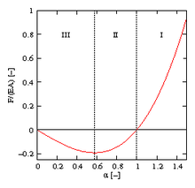
Force-extension diagram for a cylinder made of linear elastic material

The equality with the work of force results in:

${\displaystyle {\begin{aligned}\mathrm {d} W_{i}=&EV\varepsilon _{z}\mathrm {d} \varepsilon _{z}={\frac {EV}{2}}(\alpha ^{2}-1)\alpha \mathrm {d} \alpha =\mathrm {d} W_{e}=F\mathrm {d} u=FL\mathrm {d} \alpha \\\rightarrow F=&{\frac {EV}{2L}}(\alpha ^{2}-1)\alpha ={\frac {EA}{2}}(\alpha ^{2}-1)\alpha \end{aligned}}}$

The force curve is shown in the picture. In the tensile area I and in the pressure area II there is an extension α for every force , so that the system is in equilibrium. In area III the system is unstable: If the rod (its mathematical model) were loaded with, it would not find equilibrium and would collapse to zero length, which is of course unphysical. ${\displaystyle F<-{\tfrac {EA}{3{\sqrt {3}}}}=-0{,}192\,EA}$

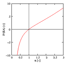
Force-extension diagram for a cylinder made of Neo-Hooke material ( K = E )

In the Neo – Hooke model the first Piola-Kirchhoff stress tensor reads P and the Cauchy stress tensor reads if a = E and with a further material parameter K ≥ E : ${\displaystyle {\boldsymbol {\sigma }}}$ ${\displaystyle k(x)=2(K-E)x+2Kx^{-1}}$

${\displaystyle {\begin{aligned}\mathbf {P} =&{\frac {\partial {\hat {W}}}{\partial \mathbf {F} }}=2E\mathbf {F} +2[K-E-K\operatorname {det} (\mathbf {F} )^{-2}]\operatorname {det} (\mathbf {F} )\mathbf {F} ^{\top -1}\\\rightarrow {\boldsymbol {\sigma }}=&{\frac {1}{\operatorname {det} (\mathbf {F} )}}\mathbf {P\cdot F} ^{\top }=2E{\begin{pmatrix}{\frac {1}{\alpha }}&&\\&{\frac {1}{\alpha }}&\\&&{\frac {\alpha }{\beta ^{2}}}\end{pmatrix}}+2\left(K-E-{\frac {K}{\alpha ^{2}\beta ^{4}}}\right){\begin{pmatrix}1&&\\&1&\\&&1\end{pmatrix}}\end{aligned}}}$

Because the radial stresses vanish, we get for the radial stretching β :

${\displaystyle {\frac {E}{\alpha }}+K-E-{\frac {K}{\alpha ^{2}\beta ^{4}}}=0\quad \rightarrow \quad \beta =\alpha ^{-{\frac {1}{2}}}\left(1+{\frac {E}{K}}{\frac {1-\alpha }{\alpha }}\right)^{-{\frac {1}{4}}}\,.}$

The parameter w in the deformation energy is adjusted so that the deformation energy in the undeformed initial state disappears at F = 1 :

${\displaystyle {\hat {W}}(\mathbf {1} )=E\|\mathbf {1} \|^{2}+(2K-2E)\operatorname {det} (\mathbf {1} )+{\frac {2K}{\operatorname {det} (\mathbf {1} )}}+w=0\quad \rightarrow \quad w=-E-4K\,.}$

The deformation energy is calculated as follows:

${\displaystyle {\begin{aligned}W_{i}=&\int _{V}\left[E\|\mathbf {F} \|^{2}+2(K-E)\operatorname {det} (\mathbf {F} )+{\frac {2K}{\operatorname {det} (\mathbf {F} )}}+w\right]\,\mathrm {d} V\\=&V\left[E(\alpha ^{2}+2\beta ^{2})+2(K-E)\alpha \beta ^{2}+{\frac {2K}{\alpha \beta ^{2}}}-E-4K\right]\end{aligned}}}$

and equilibrium with the individual force F according to d W _i = d W _e at K = E , see picture on the right:

${\displaystyle {\begin{aligned}0=&-{\frac {E}{\alpha ^{2}}}\mathrm {d} \alpha +{\frac {E}{\alpha ^{4}\beta ^{8}}}(2\alpha \mathrm {d} \alpha +4\beta ^{3}\mathrm {d} \beta )\quad \rightarrow \quad \mathrm {d} \beta =\left({\frac {\alpha \beta ^{5}}{4}}-{\frac {1}{2\beta ^{3}}}\right)\alpha \mathrm {d} \alpha \\\mathrm {d} W_{i}=&2EV\left(\alpha -{\frac {1}{\alpha ^{2}\beta ^{2}}}\right)\mathrm {d} \alpha +4EV\left(\beta -{\frac {1}{\alpha \beta ^{4}}}\right)\mathrm {d} \beta =\mathrm {d} W_{e}=FL\mathrm {d} \alpha \\\rightarrow F=&2EA\left(\alpha -{\frac {1}{\alpha ^{2}\beta ^{2}}}\right)+4EA\left(\beta -{\frac {1}{\alpha \beta ^{4}}}\right)\left({\frac {\alpha \beta ^{5}}{4}}-{\frac {1}{2\beta ^{3}}}\right)\alpha \end{aligned}}}$

Here there is a corresponding stretching for every force level and the material is stable in all areas.

Footnotes

1. ↑ To show this, we must first establish that the negative unit tensor is an element of the convex hull, for example using

   ${\displaystyle -\mathbf {1} ={\frac {1}{2}}{\begin{pmatrix}-3&&\\&1&\\&&-1\end{pmatrix}}+{\frac {1}{2}}{\begin{pmatrix}1&&\\&-3&\\&&-1\end{pmatrix}}\quad {\text{und}}\quad {\begin{vmatrix}-3&&\\&1&\\&&-1\end{vmatrix}}={\begin{vmatrix}1&&\\&-3&\\&&-1\end{vmatrix}}=3>0\,.}$

   Furthermore, the determinant of the tensor B : = λ 1 +2 A for any tensor A is a third degree polynomial in λ, which is why a positive λ can be found such that det ( B )> 0 and B then also in the convex one Shell lies. The same then also applies to the arbitrarily selectable tensor A , because: A = ½ ( λ 1 +2 A ) + ½ (- λ 1 ).
2. ↑ The Fréchet derivative of a scalar function with respect to a tensor is the tensor for which - if it exists - applies: ${\displaystyle f(\mathbf {T} )}$ ${\displaystyle \mathbf {T} }$ ${\displaystyle \mathbf {A} }$

   ${\displaystyle \mathbf {A} :\mathbf {H} =\left.{\frac {\mathrm {d} }{\mathrm {d} s}}f(\mathbf {T} +s\mathbf {H} )\right|_{s=0}=\lim _{s\rightarrow 0}{\frac {f(\mathbf {T} +s\mathbf {H} )-f(\mathbf {T} )}{s}}\quad \forall \;\mathbf {H} \,.}$

   There is and ":" the Frobenius scalar product . Then will too ${\displaystyle s\in \mathbb {R} }$

   ${\displaystyle {\frac {\partial f}{\partial \mathbf {T} }}=\mathbf {A} }$

   written.

See also

• Formula collection tensor algebra
• Tensoranalysis formula collection

literature

• JM Ball: Convexity conditions and existence theorems in non-linear elasticity . In: Archive for Rational Mechanics and Analysis . tape 63 , 1977, pp. 337-403 .
• PG Ciarlet: Mathematical Elasticity - Volume I: Three-Dimensional Elasticity . North-Holland, 1988, ISBN 0-444-70259-8 .

Individual evidence

1. ^ Paul Newton, Philip Holmes (Eds.): Geometry, Mechanics and Dynamics . Springer, 2002, ISBN 978-0-387-95518-6 , pp. 3–59 (JM Ball's post is entitled Some open problems in elasticity ).
2. ↑ Ciarlet (1988), p. 162.
3. ↑ Ciarlet (1988), pp. 185ff.
4. ^ Ciarlet (1988), p. 176
5. ↑ Ciarlet (1988), pp. 181ff
6. ↑ Ciarlet (1988), p. 189
7. ↑ Ciarlet (1988), p. 189