Taylor formula

This article deals with the Taylor formula, i.e. the representation of functions by a finite Taylor polynomial and a remainder. For the representation of functions by the limit value of the Taylor polynomials see Taylor series .

The Taylor formula (also Taylor's theorem ) is a result from the mathematical branch of analysis . It is named after the mathematician Brook Taylor . This formula can be used to approximate functions in the vicinity of a point using polynomials , the so-called Taylor polynomials . One also speaks of the Taylor approximation . The Taylor formula has become a tool in many engineering , social, and natural sciences because of its relatively simple applicability and usefulness . A complicated analytical expression can be approximated by a Taylor polynomial of low degree (often good), e.g. B. in physics or in the adjustment of geodetic networks. The often used small-angle approximation of the sine is a Taylor series of this function which is broken off after the first term.

Closely related to the Taylor formula is the so-called Taylor series (Taylor expansion ).

motivation

Approach by tangent

An approximation for a differentiable function at a point by a straight line , i.e. by a polynomial of the 1st degree, is given by the tangent to the equation ${\displaystyle f}$ ${\displaystyle a}$

${\displaystyle T_{1}f(x;a)=f(a)+f'(a)(x-a)}$.

It can be characterized in that at the location of the function values and the values of the 1st derivative (= slope) of and match: . ${\displaystyle x=a}$ ${\displaystyle f(x)}$ ${\displaystyle T_{1}f(x;a)}$ ${\displaystyle f(a)=T_{1}f(a;a),f'(a)=T_{1}'f(a;a)}$

If you define the rest , then applies . The function approximates near the point in the sense that holds for the rest ${\displaystyle R_{1}f(x;a):=f(x)-T_{1}f(x;a)}$ ${\displaystyle f(x)=T_{1}f(x;a)+R_{1}f(x;a)}$ ${\displaystyle T_{1}f(x;a)}$ ${\displaystyle f}$ ${\displaystyle x=a}$

${\displaystyle (1)~\lim _{x\to a}{\frac {R_{1}f(x;a)}{x-a}}=\lim _{x\to a}{\frac {f(x)-T_{1}f(x;a)}{x-a}}=\lim _{x\to a}{\frac {f(x)-f(a)}{x-a}}-f'(a)=0}$(see the definition of the derivative ).

Approximation by means of an osculating parabola

One can assume that one gets an even better approximation for something that is twice differentiable if one uses a quadratic polynomial , of which one demands that also hold true. The approach leads by calculating the derivatives on and , thus ${\displaystyle f}$ ${\displaystyle T_{2}f(x;a)}$ ${\displaystyle T_{2}''f(a;a)=f''(a)}$ ${\displaystyle T_{2}f(x;a)=a_{0}+a_{1}(x-a)+a_{2}(x-a)^{2}}$ ${\displaystyle a_{0}=f(a),a_{1}=f'(a)}$ ${\displaystyle a_{2}={\frac {1}{2}}f''(a)}$

${\displaystyle T_{2}f(x;a)=f(a)+f'(a)(x-a)+{\frac {1}{2}}f''(a)(x-a)^{2}}$.

This approximation function is also known as an osculating parabola.

You now define the appropriate remainder so that again . Then we get that the osculating parabola actually approximates the given function better because now (with the rule of de l'Hospital ): ${\displaystyle R_{2}f(x;a):=f(x)-T_{2}f(x;a)}$ ${\displaystyle f(x)=T_{2}f(x;a)+R_{2}f(x;a)}$ ${\displaystyle x=a}$

${\displaystyle \lim _{x\to a}{\frac {R_{2}f(x;a)}{(x-a)^{2}}}=\lim _{x\to a}{\frac {f(x)-f(a)-f'(a)(x-a)}{(x-a)^{2}}}-{\frac {1}{2}}f''(a)=\lim _{x\to a}{\frac {f'(x)-f'(a)}{2(x-a)}}-{\frac {1}{2}}f''(a)=0}$

applies.

Approximation by polynomials of degree n

This procedure can now easily be generalized to polynomials -th degree : Here should apply ${\displaystyle n}$ ${\displaystyle T_{n}(x)}$

${\displaystyle T_{n}f(a;a)=f(a),\ T_{n}'f(a;a)=f'(a),\ \ldots ,\ T_{n}^{(n)}f(a;a)=f^{(n)}(a)}$.

It turns out

${\displaystyle T_{n}f(x;a)=f(a)+{\frac {f'(a)}{1!}}(x-a)+{\frac {f''(a)}{2!}}(x-a)^{2}+\dotsb +{\frac {f^{(n)}(a)}{n!}}(x-a)^{n}}$.

With de l'Hospital's rule we also find:

${\displaystyle \lim _{x\to a}{\frac {f(x)-T_{n}f(x;a)}{(x-a)^{n}}}=\lim _{x\to a}{\frac {f'(x)-T_{n}'f(x;a)}{n(x-a)^{n-1}}}}$.

Hence with complete induction on it follows that for : ${\displaystyle n}$ ${\displaystyle R_{n}f(x;a)=f(x)-T_{n}f(x;a)}$

${\displaystyle \lim _{x\to a}{\frac {R_{n}f(x;a)}{(x-a)^{n}}}=0}$.

Qualitative Taylor formula

If -mal is differentiable, it immediately follows from the above consideration that ${\displaystyle f}$ ${\displaystyle n}$

${\displaystyle f(x)=T_{n}f(x;a)+R_{n}f(x;a)=T_{n}f(x;a)+o(|x-a|^{n}),\quad x\rightarrow a,}$

where stands for the Landau notation . This formula is called the “qualitative Taylor formula”. ${\displaystyle o}$

The closer in , the better so approximated (the so-called. Taylor polynomial, see below ) at the point the function . ${\displaystyle x}$ ${\displaystyle a}$ ${\displaystyle T_{n}f(x;a)}$ ${\displaystyle x}$ ${\displaystyle f}$

Definitions and sentence

The Taylor formula with integral remainder is presented below. The Taylor formula also exists in variants with a different remainder term; however, these formulas follow from the Taylor formula with an integral remainder term. They are listed below in the Remainder formulas section .

Let be an interval and a -time continuously differentiable function . In the following formulas stand for the first, second, ..., -th derivative of the function . ${\displaystyle I\subset \mathbb {R} }$ ${\displaystyle f\colon I\to \mathbb {R} }$ ${\displaystyle (n+1)}$ ${\displaystyle f',f'',\dots ,f^{(k)}}$ ${\displaystyle k}$ ${\displaystyle f}$

Taylor polynomial

The -th Taylor polynomial at the expansion point is defined by: ${\displaystyle n}$ ${\displaystyle a\in I}$

${\displaystyle {\begin{aligned}T_{n}f(x;a)=&\sum _{k=0}^{n}{f^{(k)}(a) \over k!}(x-a)^{k}\\=&f(a)+{\frac {f'(a)}{1!}}(x-a)+{\frac {f''(a)}{2!}}(x-a)^{2}+\ldots +{\frac {f^{(n)}(a)}{n!}}(x-a)^{n}\end{aligned}}}$

Integral remainder

The -th integral remainder is defined by: ${\displaystyle n}$

${\displaystyle R_{n}f(x;a)=\int \limits _{a}^{x}{\frac {(x-t)^{n}}{n!}}f^{(n+1)}(t)\,\mathrm {d} t}$

Theorem (Taylor formula with integral remainder term)

For everyone and off applies: ${\displaystyle a}$ ${\displaystyle x}$ ${\displaystyle I}$

${\displaystyle {\begin{aligned}f(x)=&T_{n}f(x;a)+R_{n}f(x;a)\\=&\sum _{k=0}^{n}{f^{(k)}(a) \over k!}(x-a)^{k}+\int \limits _{a}^{x}{\frac {(x-t)^{n}}{n!}}f^{(n+1)}(t)\,\mathrm {d} t\end{aligned}}}$

proof

The proof of the Taylor formula with integral remainder is done by induction over . ${\displaystyle n}$

The induction start corresponds exactly to the fundamental theorem of analysis , applied to the once continuously differentiable function : ${\displaystyle n=0}$ ${\displaystyle f}$

${\displaystyle f(x)=f(a)+\int \limits _{a}^{x}f'(t)\,\mathrm {d} t=T_{0}f(x;a)+R_{0}f(x;a)}$

The induction step (it has to be shown that the formula always holds for, if it holds for a ) takes place through partial integration . For -time continuously differentiable it results: ${\displaystyle n\rightarrow n+1}$ ${\displaystyle n+1}$ ${\displaystyle n}$ ${\displaystyle (n+2)}$ ${\displaystyle f}$

${\displaystyle {\begin{aligned}&{\frac {f^{(n+1)}(a)}{(n+1)!}}(x-a)^{n+1}+R_{n+1}f(x;a)\\=&{\frac {f^{(n+1)}(a)}{(n+1)!}}(x-a)^{n+1}+\int \limits _{a}^{x}{\frac {(x-t)^{n+1}}{(n+1)!}}f^{(n+2)}(t)\,\mathrm {d} t\\=&{\frac {f^{(n+1)}(a)}{(n+1)!}}(x-a)^{n+1}+\left[{\frac {(x-t)^{n+1}}{(n+1)!}}f^{(n+1)}(t)\right]_{t=a}^{t=x}-\int \limits _{a}^{x}{\frac {-(x-t)^{n}}{n!}}f^{(n+1)}(t)\,\mathrm {d} t\\=&{\frac {(x-a)^{n+1}}{(n+1)!}}f^{(n+1)}(a)-{\frac {(x-a)^{n+1}}{(n+1)!}}f^{(n+1)}(a)+R_{n}f(x;a)\\=&R_{n}f(x;a)\end{aligned}}}$

and thus

${\displaystyle T_{n+1}f(x;a)+R_{n+1}f(x;a)=T_{n}f(x;a)+R_{n}f(x;a)=f(x)}$.

Remainder formulas

Besides the integral formula, there are other representations of the remainder of the term.

Schlömilch residual link and its derivation

According to the mean value theorem of integral calculus, it follows for every natural number with that there is an between and so that: ${\displaystyle p}$ ${\displaystyle 1\leq p\leq n+1}$ ${\displaystyle \xi }$ ${\displaystyle a}$ ${\displaystyle x}$

${\displaystyle \int \limits _{a}^{x}{f^{(n+1)}(t){\frac {(x-t)^{n+1-p}}{n!}}\cdot (x-t)^{p-1}\,\mathrm {d} t}={\frac {f^{(n+1)}(\xi )(x-\xi )^{n+1-p}}{n!}}\cdot \underbrace {\int \limits _{a}^{x}{(x-t)^{p-1}\,\mathrm {d} t}} _{={\frac {(x-a)^{p}}{p}}}}$

This follows the Schlömilch residual limb form :

${\displaystyle R_{n}f(x;a)=\int \limits _{a}^{x}{\frac {(x-t)^{n}}{n!}}f^{(n+1)}(t)\,\mathrm {d} t={\frac {f^{(n+1)}(\xi )}{p\cdot n!}}(x-\xi )^{n+1-p}(x-a)^{p}}$

for a between and . ${\displaystyle \xi }$ ${\displaystyle a}$ ${\displaystyle x}$

Special cases of the Schlömilch residual limb

A special case, namely the one with , is the Cauchy form : ${\displaystyle p=1}$

${\displaystyle R_{n}f(x;a)={\frac {f^{(n+1)}(\xi )}{n!}}(x-\xi )^{n}(x-a)}$

for a between and . ${\displaystyle \xi }$ ${\displaystyle a}$ ${\displaystyle x}$

In the special case we get the Lagrangian remainder : ${\displaystyle p=n+1}$

${\displaystyle R_{n}f(x;a)={\frac {f^{(n+1)}(\xi )}{(n+1)!}}(x-a)^{n+1}}$

for a between and . In this representation, the -th derivative of need not be continuous. ${\displaystyle \xi }$ ${\displaystyle a}$ ${\displaystyle x}$ ${\displaystyle (n+1)}$ ${\displaystyle f}$

Peano residual link

With the Taylor formula with Lagrange remainder one obtains for -mal continuously differentiable also: ${\displaystyle n}$ ${\displaystyle f}$

${\displaystyle f(x)=T_{n-1}f(x;a)+{\frac {f^{(n)}(\xi )}{n!}}(x-a)^{n}=T_{n}f(x;a)+{\frac {f^{(n)}(\xi )-f^{(n)}(a)}{n!}}(x-a)^{n}}$

That’s why you can as a remainder

${\displaystyle R_{n}f(x;a)={\frac {f^{(n)}(\xi )-f^{(n)}(a)}{n!}}(x-a)^{n}}$

use, with only times must be continuously differentiable. This remainder is called a Peano remainder . ${\displaystyle f}$ ${\displaystyle n}$

Further representation

If one sets , that is , the Lagrangian representation receives the form ${\displaystyle \Theta ={\tfrac {\xi -a}{x-a}}}$ ${\displaystyle \xi =a+\Theta (x-a)}$

${\displaystyle R_{n}f(x;a)={\frac {f^{(n+1)}(a+\Theta (x-a))}{(n+1)!}}(x-a)^{n+1}}$,

the Schlömilchsche

${\displaystyle R_{n}f(x;a)={\frac {f^{(n+1)}(a+\Theta (x-a))}{p\cdot n!}}(1-\Theta )^{n+1-p}(x-a)^{n+1}}$,

and the Cauchysche

${\displaystyle R_{n}f(x;a)={\frac {f^{(n+1)}(a+\Theta (x-a))}{n!}}(1-\Theta )^{n}(x-a)^{n+1}}$

each for one between 0 and 1. ${\displaystyle \Theta }$

Residual link estimation

If the interval is in (the domain of ), one can derive the following estimate with the remainder of Lagrange (see in the section remainder formulas ) for all and because of between and (and thus also ): ${\displaystyle (a-r,a+r)}$ ${\displaystyle I}$ ${\displaystyle f}$ ${\displaystyle x\in (a-r,a+r)}$ ${\displaystyle \xi }$ ${\displaystyle a}$ ${\displaystyle x}$ ${\displaystyle \xi \in (a-r,a+r)}$

${\displaystyle |R_{n}f(x;a)|=\left|{\frac {f^{(n+1)}(\xi )}{(n+1)!}}(x-a)^{n+1}\right|\leq \sup _{\xi \in (a-r,a+r)}\left|{\frac {f^{(n+1)}(\xi )}{(n+1)!}}(x-a)^{n+1}\right|}$

If it applies to all , then the estimate applies to the remainder of the term ${\displaystyle |f^{(n+1)}(x)|\leq M_{n}}$ ${\displaystyle x\in (a-r,a+r)}$

${\displaystyle \forall x\in (a-r,a+r):|R_{n}f(x;a)|\leq M_{n}{\frac {|x-a|^{n+1}}{(n+1)!}}\leq M_{n}{\frac {r^{n+1}}{(n+1)!}}}$.

Approximation formulas for sine and cosine

One application of the Taylor formula are approximation formulas, presented here using the example of sine and cosine (where the argument is given in radians ).

For , the 4th Taylor polynomial of the sine function at the expansion point is 0 ${\displaystyle f(x)=\sin(x)}$ ${\displaystyle f'(x)=\cos(x),\,f''(x)=-\sin(x),\,f'''(x)=-\cos(x),f''''(x)=\sin(x)}$

${\displaystyle T_{4}\sin(x;0)=f(0)+f'(0)x+{\frac {1}{2}}f''(0)x^{2}+{\frac {1}{6}}f'''(0)x^{3}+{\frac {1}{24}}f''''(0)x^{4}=x-{\frac {x^{3}}{6}}.}$

From results for the remainder of Lagrange with between 0 and . Due to the remainder of the term . ${\displaystyle f^{(5)}(x)=\cos(x)}$ ${\displaystyle R_{4}\sin(x;0)={\frac {f^{(5)}(\xi )}{5!}}x^{5}={\frac {\cos(\xi )}{120}}x^{5}}$ ${\displaystyle \xi }$ ${\displaystyle x}$ ${\displaystyle |{\cos(\xi )}|\leq 1}$ ${\displaystyle |T_{4}\sin(x;0)-\sin(x)|\leq {\frac {|x|^{5}}{120}}}$

If it is between and , the relative deviation from to is less than 0.5%. ${\displaystyle x}$ ${\displaystyle -{\frac {\pi }{4}}}$ ${\displaystyle {\frac {\pi }{4}}}$ ${\displaystyle \left|{\frac {T_{4}\sin(x;0)-\sin(x)}{\sin(x)}}\right|}$ ${\displaystyle T_{3}\sin(x;0)}$ ${\displaystyle \sin(x)}$

In fact, the 3rd order Taylor polynomial is sufficient for approximating the sine to this accuracy, since for , and therefore . This also results in the following further estimate for the third and fourth Taylor polynomial, which is more precise for very large x: ${\displaystyle f''''(0)=0}$ ${\displaystyle f(x)=\sin(x)}$ ${\displaystyle T_{3}\sin(x;0)=T_{4}\sin(x;0)}$

${\displaystyle |T_{4}\sin(x;0)-\sin(x)|\leq {\frac {x^{4}}{24}}}$

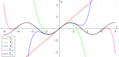
The following figure shows the graphs of some Taylor polynomials of the sine around development point 0 for . The graph to belongs to the Taylor series , which corresponds to the sine function. ${\displaystyle n=1,3,5,15}$ ${\displaystyle n=\infty }$

Approximation of the sine by Taylor polynomials to ${\displaystyle T_{1}\sin(x;0)}$ ${\displaystyle T_{81}\sin(x;0)}$

The fourth Taylor polynomial of the cosine function at the expansion point 0 has this form in the Horner scheme : ${\displaystyle T_{4}\cos(x;0)}$

${\displaystyle \cos(x)\approx T_{4}\cos(x;0)=\left({\frac {x^{2}}{12}}-1\right)\cdot {\frac {x^{2}}{2}}+1}$

If x is between and , the relative deviation is less than 0.05%. ${\displaystyle -{\frac {\pi }{4}}}$ ${\displaystyle {\frac {\pi }{4}}}$ ${\displaystyle \left|{\frac {T_{4}\cos(x;0)-\cos(x)}{\cos(x)}}\right|}$

You can also use these formulas for cotangent and tangent , because it is

${\displaystyle \tan(x)\sim t(x)={\frac {T_{3}\sin(x;0)}{T_{4}\cos(x;0)}}}$

with a relative deviation of less than 0.5% for , and with the same relative deviation (there is no Taylor polynomial of the tangent). ${\displaystyle \left|x\right|<{\frac {\pi }{4}}}$ ${\displaystyle \cot(x)\sim 1/t(x)}$ ${\displaystyle t}$

If you need an even higher accuracy for your approximation formulas, you can fall back on higher Taylor polynomials, which approximate the functions even better.

Taylor formula in the multidimensional

See also : “Multidimensional Taylor Series” in the Taylor Series article

In the following, let us be a -time continuously differentiable function and . Is further , wherein . ${\displaystyle f\colon \mathbb {R} ^{d}\to \mathbb {R} }$ ${\displaystyle n+1}$ ${\displaystyle x=(x_{1},\ldots ,x_{d}),a=(a_{1},\ldots ,a_{d})\in \mathbb {R} ^{d}}$ ${\displaystyle F\colon \mathbb {R} \to \mathbb {R} }$ ${\displaystyle F(t)=f(a+th)}$ ${\displaystyle h=x-a}$

Furthermore, be as in the multi-index notation . In the following section, the multi-index notation is used so that one can immediately see that the multi-dimensional case actually results in the same formulas as the one-dimensional case. ${\displaystyle D^{\alpha }={\frac {\partial ^{|\alpha |}}{\partial x_{1}^{\alpha _{1}}\cdots \partial x_{d}^{\alpha _{d}}}}}$ ${\displaystyle d=1}$

Multi-dimensional Taylor polynomial

With the multidimensional chain rule and induction we get that

${\displaystyle F^{(n)}(t)=\sum _{|\alpha |=n}\left({\begin{matrix}n\\\alpha \end{matrix}}\right)(x-a)^{\alpha }D^{\alpha }f(a+th)}$,

where is the multinomial coefficient, see multinomial theorem . ${\displaystyle \left({\begin{matrix}n\\\alpha \end{matrix}}\right)}$

If you represent a Taylor polynomial with development point 0 at point 1, this formula gives the definition of the multi-dimensional Taylor polynomial of at the development point : ${\displaystyle F}$ ${\displaystyle f}$ ${\displaystyle a}$

${\displaystyle T_{n}f(x;a):=T_{n}F(1;0)=\sum _{|\alpha |=0}^{n}{\frac {(x-a)^{\alpha }}{\alpha !}}D^{\alpha }f(a)}$

Here it was used that . ${\displaystyle \left({\begin{matrix}n\\\alpha \end{matrix}}\right)\cdot {\frac {1}{n!}}={\frac {1}{\alpha !}}}$

Oscillating quadric

The second Taylor polynomial of a scalar-valued function in more than one variable can be written more compactly up to the second order than:

${\displaystyle T_{2}f(x;a)=f(a)+\nabla f(a)^{T}(x-a)+{\frac {1}{2}}(x-a)^{T}\operatorname {H} _{f}(a)(x-a)}$

Here, the gradient and the Hessian matrix of each at the site . ${\displaystyle \nabla f(a)}$ ${\displaystyle \operatorname {H} _{f}(a)}$ ${\displaystyle f}$ ${\displaystyle a}$

The second Taylor polynomial is also called an oscillating quadric .

Multi-dimensional integral remainder

The multidimensional remainder of the term is also defined using the multi-index notation:

${\displaystyle {\begin{aligned}R_{n}f(x;a):=&R_{n}F(1;0)=\int \limits _{0}^{1}{\frac {(1-t)^{n}}{n!}}F^{(n+1)}(t)\,\mathrm {d} t\\=&(n+1)\int \limits _{0}^{1}\sum _{|\alpha |=n+1}{\frac {(1-t)^{n}(x-a)^{\alpha }}{\alpha !}}D^{\alpha }f(a+th)\,\mathrm {d} t\end{aligned}}}$

Multi-dimensional Taylor formula

From the one-dimensional Taylor formula it follows that

${\displaystyle F(1)=T_{n}F(1;0)+R_{n}F(1;0)}$

Therefore, according to the definition of above , one obtains: ${\displaystyle F(t)}$

${\displaystyle f(x)=T_{n}f(x;a)+R_{n}f(x;a)}$

Multi-dimensional remainder formulas

The one-dimensional non-integral residual term formulas can also be generalized for the multidimensional case using the formula for . ${\displaystyle F^{(n)}(t)}$

The Schlömilch remainder becomes like this

${\displaystyle R_{n}f(x;a)={\frac {(n+1)(1-\theta )^{n+1-p}}{p}}\sum _{|\alpha |=n+1}{\frac {(x-a)^{\alpha }D^{\alpha }f(a+\theta h)}{\alpha !}}}$,

the Lagrangian remainder

${\displaystyle R_{n}f(x;a)=\sum _{|\alpha |=n+1}{\frac {(x-a)^{\alpha }D^{\alpha }f(a+\theta h)}{\alpha !}}}$,

and the Cauchy remainder

${\displaystyle R_{n}f(x;a)=(n+1)(1-\theta )^{n}\sum _{|\alpha |=n+1}{\frac {(x-a)^{\alpha }D^{\alpha }f(a+\theta h)}{\alpha !}}}$

for each one . ${\displaystyle \theta \in [0,1]}$

Qualitative Taylor formula

According to the multidimensional Taylor formula with the Lagrange remainder, we get:

${\displaystyle f(x)-T_{n+1}f(x;a)=(n+1)\left(\sum _{|\alpha |=n+1}{\frac {(x-a)^{\alpha }D^{\alpha }f(a+\theta h)}{\alpha !}}-\sum _{|\alpha |=n+1}{\frac {(x-a)^{\alpha }D^{\alpha }f(a)}{\alpha !}}\right)}$

Because we get further: ${\displaystyle |x_{i}-a_{i}|\leq \|x-a\|}$

${\displaystyle {\begin{aligned}&(n+1)\left|\sum _{|\alpha |=n+1}{\frac {(x-a)^{\alpha }D^{\alpha }f(a+\theta h)}{\alpha !}}-\sum _{|\alpha |=n+1}{\frac {(x-a)^{\alpha }D^{\alpha }f(a)}{\alpha !}}\right|\\\leq &(n+1)\|x-a\|^{n+1}\cdot \underbrace {\left|\sum _{|\alpha |=n+1}{\frac {D^{\alpha }f(a+\theta h)-D^{\alpha }f(a)}{\alpha !}}\right|} _{\to 0{\text{, }}x\to a}\end{aligned}}}$

The last part tends to zero, since the partial derivatives of the degree are all continuous and are located between and and thus also converge to, if . ${\displaystyle n+1}$ ${\displaystyle a+\theta h}$ ${\displaystyle x}$ ${\displaystyle a}$ ${\displaystyle a}$ ${\displaystyle x\to a}$

We get the following estimate, which is called the "(multidimensional) qualitative Taylor formula":

${\displaystyle f(x)=T_{n+1}f(x;a)+{\mathcal {O}}(\|x-a\|^{n+1})}$

for , where stands for Landau notation . ${\displaystyle x\to a}$ ${\displaystyle {\mathcal {O}}}$

example

It's supposed to function

${\displaystyle f:\{(x_{1},x_{2})\in \mathbb {R} ^{2},\ x_{2}<1\}\to \mathbb {R} ,~(x_{1},x_{2})\mapsto \exp(x_{1}-x_{2})\cdot \log(1-x_{2})}$

to be developed around the point . ${\displaystyle a=(a_{1},a_{2})=(1,0)\in \mathbb {R} ^{2}}$

Function (red) and Taylor expansion (green)

In this example, the function is to be developed up to the second degree, that is, one wants to calculate a second order Taylor polynomial, the so-called oscillation quadric . So it applies . Because of need, according to the multi-index notation , the tuples , , , , and are taken into account. Because of Schwarz's theorem, it holds that ${\displaystyle n=2}$ ${\displaystyle |\alpha |\leq n}$ ${\displaystyle (0,0)}$ ${\displaystyle (1,0)}$ ${\displaystyle (0,1)}$ ${\displaystyle (2,0)}$ ${\displaystyle (1,1)}$ ${\displaystyle (0,2)}$

${\displaystyle {\frac {\partial ^{2}f}{\partial x_{1}\partial x_{2}}}(a)={\frac {\partial ^{2}f}{\partial x_{2}\partial x_{1}}}(a)}$.

The partial derivatives of the function are:

${\displaystyle {\frac {\partial f}{\partial x_{1}}}(a)=\left[\exp(x_{1}-x_{2})\cdot \log(1-x_{2})\right]_{x=(1,0)}=0}$

${\displaystyle {\frac {\partial f}{\partial x_{2}}}(a)=\left[-\exp(x_{1}-x_{2})\cdot \left(\log(1-x_{2})+{\frac {1}{1-x_{2}}}\right)\right]_{x=(1,0)}=-e}$

${\displaystyle {\frac {\partial ^{2}f}{\partial x_{1}^{2}}}(a)=\left[\exp(x_{1}-x_{2})\cdot \log(1-x_{2})\right]_{x=(1,0)}=0}$

${\displaystyle {\frac {\partial ^{2}f}{\partial x_{1}\partial x_{2}}}(a)={\frac {\partial ^{2}f}{\partial x_{2}\partial x_{1}}}(a)=\left[-\exp(x_{1}-x_{2})\cdot \left(\log(1-x_{2})+{\frac {1}{1-x_{2}}}\right)\right]_{x=(1,0)}=-e}$

${\displaystyle {\frac {\partial ^{2}f}{\partial x_{2}^{2}}}(a)=\left[\exp(x_{1}-x_{2})\left(\log(1-x_{2})+{\frac {2}{1-x_{2}}}-{\frac {1}{(1-x_{2})^{2}}}\right)\right]_{x=(1,0)}=e}$

It follows with the multi-dimensional Taylor formula:

${\displaystyle {\begin{aligned}f(x)\approx &f(a)+{\frac {1}{1!}}{\frac {\partial f}{\partial x_{1}}}(a)~(x_{1}-a_{1})+{\frac {1}{1!}}{\frac {\partial f}{\partial x_{2}}}(a)~(x_{2}-a_{2})\\&+{\frac {1}{2!}}{\frac {\partial ^{2}f}{\partial x_{1}^{2}}}(a)~(x_{1}-a_{1})^{2}+{\frac {1}{1!1!}}{\frac {\partial ^{2}f}{\partial x_{1}\partial x_{2}}}(a)~(x_{1}-a_{1})(x_{2}-a_{2})\\&+{\frac {1}{2!}}{\frac {\partial ^{2}f}{\partial x_{2}^{2}}}(a)~(x_{2}-a_{2})^{2}\\&=0+0-e(x_{2}-0)+0-e(x_{1}-1)(x_{2}-0)+{\frac {1}{2}}e(x_{2}-0)^{2}\\&=-ex_{1}x_{2}+{\frac {1}{2}}ex_{2}^{2}\end{aligned}}}$

If you use the alternative representation with the help of the gradient and the Hessian matrix, you get:

${\displaystyle {\begin{aligned}f(x)&\approx f(a)+\nabla f(a)^{T}(x-a)+{\frac {1}{2}}(x-a)^{T}H_{f}(a)(x-a)\\&=f(a)+{\begin{pmatrix}{\frac {\partial f}{\partial x_{1}}}(a)&{\frac {\partial f}{\partial x_{2}}}(a)\end{pmatrix}}{\begin{pmatrix}x_{1}-a_{1}\\x_{2}-a_{2}\end{pmatrix}}\\&\qquad +{\frac {1}{2}}{\begin{pmatrix}x_{1}-a_{1}&x_{2}-a_{2}\end{pmatrix}}{\begin{pmatrix}{\frac {\partial ^{2}f}{\partial x_{1}^{2}}}(a)&{\frac {\partial ^{2}f}{\partial x_{2}\partial x_{1}}}(a)\\{\frac {\partial ^{2}f}{\partial x_{1}\partial x_{2}}}(a)&{\frac {\partial ^{2}f}{\partial x_{2}^{2}}}(a)\end{pmatrix}}{\begin{pmatrix}x_{1}-a_{1}\\x_{2}-a_{2}\end{pmatrix}}\\&=0+{\begin{pmatrix}0&-e\end{pmatrix}}{\begin{pmatrix}x_{1}-1\\x_{2}\end{pmatrix}}+{\frac {1}{2}}{\begin{pmatrix}x_{1}-1&x_{2}\end{pmatrix}}{\begin{pmatrix}0&-e\\-e&e\end{pmatrix}}{\begin{pmatrix}x_{1}-1\\x_{2}\end{pmatrix}}\\&=-ex_{1}x_{2}+{\frac {1}{2}}ex_{2}^{2}\end{aligned}}}$

literature

• Otto Forster : Analysis. Volume 1: Differential and integral calculus of a variable. 8th, improved edition. Vieweg + Teubner, Wiesbaden 2006, ISBN 3-8348-0088-0 ( Vieweg study. Basic course in mathematics ).
• Otto Forster: Analysis. Volume 2: differential calculus in R ⁿ . Ordinary differential equations. 7th, improved edition. Vieweg + Teubner, Wiesbaden 2006, ISBN 3-8348-0250-6 ( Vieweg study. Basic course in mathematics ).
• Bernhard Heck : Calculation methods and evaluation models for national surveying. Classic and modern methods. Wichmann, Karlsruhe 1987, ISBN 3-87907-173-X , Chapters 4, 7 and 13 (Mathematical Models and Fundamentals).
• Konrad Königsberger : Analysis. Volume 2. 3rd, revised edition. Springer, Berlin et al. 2000, ISBN 3-540-66902-7 .

Individual evidence

1. ↑ Brook Taylor: Methodus Incrementorum Directa et Inversa. Pearson, London 1717, p. 21 .
2. ^ Königsberger: Analysis. Volume 2. 2000, p. 66.