Sine and cosine

Sine, Cosine and Cosine are redirects to this article. For further meanings, see Sine (disambiguation) , Cosine (disambiguation) and Cosine (disambiguation) .

Graphs of the sine function (red) and the cosine function (blue). Both functions have a period of and take values ​​from −1 to 1. ${\displaystyle 2\pi }$

Sine and cosine functions (also known as cosine functions ) are elementary mathematical functions . They form the most important trigonometric functions before the tangent and cotangent , secant and cosecant . Sine and cosine are required, among other things, in geometry for triangular calculations in plane and spherical trigonometry . They are also important in analysis .

Waves such as sound waves , water waves and electromagnetic waves can be described as a combination of sine and cosine waves , so that the functions are omnipresent in physics as harmonic oscillations .

origin of the name

Gerhard von Cremona chose the Latin term sinus "bow, curvature, bosom" for this mathematical term in 1175 as a translation of the Arabic term gaib or jiba (جيب) "bag, fold of clothes", borrowed from Sanskrit jiva "bowstring" by Indian mathematicians.

The term "cosine" results from complementi sinus, that is, the sine of the complementary angle . This term was first used in the extensive trigonometric tables created by Georg von Peuerbach and his student Regiomontanus .

Geometric definition

Definition on the right triangle

Triangle with points ABC and opposite sides a, b, c

Triangle ABC with a right angle in C. (Designation of the on and opposite cathets, assuming that the angle under consideration is.) ${\displaystyle \gamma }$ ${\displaystyle \alpha }$

All flat, similar triangles have the same angles and the same length ratios of the sides .

This property is used to perform calculations on a right triangle . If the length ratios in the right triangle are known, the dimensions of angles and lengths of sides can be calculated. That is why the length ratios in the right triangle have special names.

The length ratios of the three sides in the right triangle are only dependent on the size of the two acute angles . Because the inside angle sum in each triangle is 180 °. And because an angle in a right-angled triangle, namely the right angle, is known to be 90 °, the other two angles must also add up to 90 °. Therefore the dimension of one of these angles is already determined by the dimension of the other angle. Due to the triangular sets (e.g. WSW), the length ratios in a right-angled triangle only depend on the size of one of the two acute angles.

Therefore the length ratios are defined as follows depending on one of the two acute angles:

The sine of an angle is the ratio of the length of the opposite cathetus ( cathetus opposite the angle) to the length of the hypotenuse (side opposite the right angle).

${\displaystyle {\text{Sinus eines Winkels}}={\frac {\text{Gegenkathete des Winkels}}{\text{Hypotenuse}}}}$

The cosine is the ratio of the length of the adjacent cathetus (that is, the cathetus that forms one leg of the angle) to the length of the hypotenuse.

${\displaystyle {\text{Kosinus eines Winkels}}={\frac {\text{Ankathete des Winkels}}{\text{Hypotenuse}}}}$

With the usual designations of the sizes for triangles (see illustration) the following applies here:

${\displaystyle \sin(\alpha )={\frac {a}{c}}\quad {\text{und}}\quad \cos(\alpha )={\frac {b}{c}}}$

Since the hypotenuse is the longest side of a triangle (because it lies opposite the largest angle, i.e. the right angle), the inequalities and apply . ${\displaystyle \sin \left(\alpha \right)\leq 1}$ ${\displaystyle \cos \left(\alpha \right)\leq 1}$

If the opposite angle β is assumed instead of α, then both sides change their role, the adjacent side of α becomes the opposite side of β and the opposite side of α now forms the side of β and the following applies:

${\displaystyle \sin(\beta )={\frac {b}{c}}}$

${\displaystyle \cos(\beta )={\frac {a}{c}}}$

Since in a right triangle it follows: ${\displaystyle \alpha +\beta =90^{\circ }}$

${\displaystyle \cos(\alpha )=\sin(90^{\circ }-\alpha )=\sin(\beta )}$

and

${\displaystyle \sin(\alpha )=\cos(90^{\circ }-\alpha )=\cos(\beta )}$

The designation cosine as the sine of the complementary angle is based on this relationship .

From the Pythagorean theorem , the relationship ( "leaves trigonometric Pythagoras ") derived:

${\displaystyle \sin ^{2}\left(\alpha \right)+\cos ^{2}\left(\alpha \right)=1}$

In the right triangle, sine and cosine are only defined for angles between 0 and 90 degrees. For any angle, the value of the sine function is defined as the coordinate and the value of the cosine function as the coordinate of a point on the unit circle ( see below ). Here it is common to use the value to which the function is applied (here: the angle) as an argument . This applies in particular to the trigonometric functions and the complex exponential function ( see below ). ${\displaystyle y}$ ${\displaystyle x}$

Definition on the unit circle

Definition of the sine and cosine on the unit circle

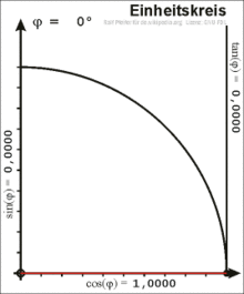
Trigonometric functions on the unit circle in the first quadrant

In the right triangle, the angle between the hypotenuse and the cathetus is only defined for values ​​from 0 to 90 degrees. For a general definition, a point with the coordinates on the unit circle is considered, here the following applies . The positive axis encloses an angle with the position vector of . The origin of coordinates , the point on the axis and the point form a right triangle. The length of the hypotenuse is . The adjacent side of the angle is the distance between and and has the length . The following applies: ${\displaystyle P}$ ${\displaystyle (x,y)}$ ${\displaystyle x^{2}+y^{2}=1}$ ${\displaystyle x}$ ${\displaystyle P}$ ${\displaystyle \alpha }$ ${\displaystyle (0,0)}$ ${\displaystyle (x,0)}$ ${\displaystyle x}$ ${\displaystyle P(x,y)}$ ${\displaystyle {\sqrt {x^{2}+y^{2}}}=1}$ ${\displaystyle \alpha }$ ${\displaystyle (0,0)}$ ${\displaystyle (x,0)}$ ${\displaystyle |x|}$

${\displaystyle \cos(\alpha )=x}$.

The opposite side of the angle is the distance between and and has the length . Thus: ${\displaystyle \alpha }$ ${\displaystyle (x,0)}$ ${\displaystyle (x,y)}$ ${\displaystyle |y|}$

${\displaystyle \sin(\alpha )=y}$.

From this the definition of the tangent follows through the theorem of rays :

${\displaystyle \tan \alpha ={\frac {\sin \alpha }{\cos \alpha }}}$.

The coordinate of a point in the first quadrant of the unit circle is the sine of the angle between its position vector and the axis, while the coordinate is the cosine of the angle. Continuing beyond the first quadrant results in a definition of sine and cosine for any angle. ${\displaystyle y}$ ${\displaystyle x}$ ${\displaystyle x}$

The inverse of the sine / cosine function is not unique. For every number between −1 and 1 ( ) there are always exactly two angles between 0 ° and 360 ° ( ). The symmetries of the trigonometric functions can be recognized by the following relationships: ${\displaystyle y}$ ${\displaystyle -1<y<1}$ ${\displaystyle 0^{\circ }<\alpha \leq 360^{\circ }}$

Point symmetries:

${\displaystyle \sin(-\alpha )=-\sin(\alpha )}$

and

${\displaystyle \cos(90^{\circ }+\alpha )=-\cos(90^{\circ }-\alpha )}$,

Axis symmetries:

${\displaystyle \cos(-\alpha )=\cos(\alpha )}$

and

${\displaystyle \sin(90^{\circ }+\alpha )=\sin(90^{\circ }-\alpha )}$ .

The sinus is thus an odd function of the cosine of a straight .

Sine and cosine are periodic functions with a period of 360 degrees. (You cannot distinguish an angle of 365 °, for example, from an angle of 5 °. But one describes a rotary movement of just over one turn, the other a very small rotary movement - only a seventy-second turn.) So also applies

${\displaystyle \sin(\alpha +k\cdot 360^{\circ })=\sin(\alpha )}$

such as

${\displaystyle \cos(\alpha +k\cdot 360^{\circ })=\cos(\alpha )}$,

where is any integer. So there are not only the symmetries to (cos) or (sin) and to (sin) or (cos), but an infinite number of axes of symmetry and centers of symmetry for both functions. ${\displaystyle k}$ ${\displaystyle \alpha =0^{\circ }}$ ${\displaystyle \alpha =90^{\circ }}$ ${\displaystyle (0,0)}$ ${\displaystyle (90^{\circ }|0)}$

The following animation illustrates the emergence of the sine and cosine functions from the rotary movement of an angled limb starting at the axis. The angle is measured in radians . An angle of corresponds to a radian measure of . ${\displaystyle x}$ ${\displaystyle 360^{\circ }}$ ${\displaystyle 2\pi }$

Analytical definition

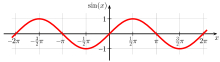
Graph of the sine function ${\displaystyle x\mapsto \sin(x)}$

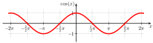
Graph of the cosine function ${\displaystyle x\mapsto \cos(x)}$

Sine and cosine can also be treated on an axiomatic basis; this more formal approach also plays a role in analysis . The analytical definition also allows expansion to include complex arguments. Sin and cosine as complex-valued functions are holomorphic and surjective .

Motivation by Taylor series

${\displaystyle \cos(x)}$ together with the first Taylor polynomials ${\displaystyle p_{n}(x)=\sum _{k=0}^{n}(-1)^{k}{\frac {x^{2k}}{(2k)!}}}$

This animation illustrates the definition of the sine function through a series. The higher the number , the more summands are used in the series definition. In addition to the sine function, the cubic polynomial is also drawn in. ${\displaystyle N}$ ${\displaystyle N=2}$ ${\displaystyle \sum _{k=0}^{2}{\tfrac {(-1)^{k}}{(2k+1)!}}x^{2k+1}=x-{\tfrac {x^{3}}{6}}}$

Due to the transition from angle to radian , sine and cosine can be explained as functions from to . It can be shown that they can be differentiated any number of times. The following applies to the derivatives at zero: ${\displaystyle \mathbb {R} }$ ${\displaystyle \mathbb {R} }$

${\displaystyle \sin ^{(4n+k)}(0)=\left\{{\begin{matrix}0&{\text{wenn }}k=0\\1&{\text{wenn }}k=1\\0&{\text{wenn }}k=2\\-1&{\text{wenn }}k=3\end{matrix}}\right.\qquad \cos ^{(4n+k)}(0)=\left\{{\begin{matrix}1&{\text{wenn }}k=0\\0&{\text{wenn }}k=1\\-1&{\text{wenn }}k=2\\0&{\text{wenn }}k=3\end{matrix}}\right.}$.

The choice of radian means that the values appear here. The resulting Taylor series represent the functions and , that is: ${\displaystyle \pm 1}$ ${\displaystyle \sin(x)}$ ${\displaystyle \cos(x)}$

${\displaystyle \sin(x)=\sum _{n=0}^{\infty }(-1)^{n}{\frac {x^{2n+1}}{(2n+1)!}}={\frac {x}{1!}}-{\frac {x^{3}}{3!}}+{\frac {x^{5}}{5!}}\mp \dotsb }$

${\displaystyle \cos(x)=\sum _{n=0}^{\infty }(-1)^{n}{\frac {x^{2n}}{(2n)!}}={\frac {x^{0}}{0!}}-{\frac {x^{2}}{2!}}+{\frac {x^{4}}{4!}}\mp \dotsb }$

Series development in analysis

In analysis one starts from a series expansion and, conversely, derives everything from it by explaining the functions sin and cos by the power series given above . With the quotient criterion it can be shown that these power series converge evenly for every complex number absolutely and in every restricted subset of the complex numbers . These infinite series generalize the definition of sine and cosine from real to complex arguments. Also there is usually not defined geometrically, but for example via the cos series and the relationship as twice the smallest positive zero of the cosine function. This gives a precise analytical definition of . ${\displaystyle x}$ ${\displaystyle \pi }$ ${\displaystyle \cos \left({\tfrac {\pi }{2}}\right)=0}$ ${\displaystyle \pi }$

For small values, these series show very good convergence behavior. The periodicity and symmetry of the functions can therefore be used for numerical calculation and the value can be reduced to the range to . Then only a few terms of the series have to be calculated for the required accuracy. The Taylor polynomial of the cosine function to the fourth power z. B. has a relative error of less than 0.05% in the interval . In the Taylor formula article , some of these so-called Taylor polynomials are shown graphically and an approximation formula is given with details of the accuracy. It should be noted, however, that the partial sums of the Taylor polynomials do not represent the best possible numerical approximation; For example, in Abramowitz-Stegun there are approximation polynomials with even smaller approximation errors. ${\displaystyle x}$ ${\displaystyle -\pi /4}$ ${\displaystyle \pi /4}$ ${\displaystyle [-\pi /4,\pi /4]}$

Relationship to the exponential function

The real part of is and the imaginary part is ${\displaystyle \mathrm {e} ^{\mathrm {i} \theta }}$ ${\displaystyle \cos \theta }$ ${\displaystyle \sin \theta }$

The trigonometric functions are closely related to the exponential function , as the following calculation shows:

${\displaystyle {\begin{aligned}\mathrm {e} ^{\mathrm {i} x}&=\sum _{k=0}^{\infty }{\frac {(\mathrm {i} x)^{k}}{k!}}=\sum _{l=0}^{\infty }{\frac {(\mathrm {i} x)^{2l}}{(2l)!}}+\sum _{l=0}^{\infty }{\frac {(\mathrm {i} x)^{2l+1}}{(2l+1)!}}\\&=\underbrace {\sum _{l=0}^{\infty }(-1)^{l}{\frac {x^{2l}}{(2l)!}}} _{\cos x}+\mathrm {i} \underbrace {\sum _{l=0}^{\infty }(-1)^{l}{\frac {x^{2l+1}}{(2l+1)!}}} _{\sin x}\\&=\cos x+\mathrm {i} \sin x\end{aligned}}}$

It was used as well ${\displaystyle \mathrm {i} ^{2l}=(\mathrm {i} ^{2})^{l}=(-1)^{l}\,}$ ${\displaystyle \mathrm {i} ^{2l+1}=\mathrm {i} \cdot \mathrm {i} ^{2l}=\mathrm {i} (-1)^{l}}$

Relationship between sine, cosine and exponential function

This results in the so-called Euler formula

${\displaystyle \mathrm {e} ^{\mathrm {i} x}=\cos x+\mathrm {i} \cdot \sin x}$.

So for a real number is the real part and the imaginary part of the complex number . ${\displaystyle x}$ ${\displaystyle \cos(x)}$ ${\displaystyle \sin(x)}$ ${\displaystyle \mathrm {e} ^{\mathrm {i} x}}$

Replacing with results in: ${\displaystyle x}$ ${\displaystyle -x}$

${\displaystyle \mathrm {e} ^{-\mathrm {i} x}=\cos x-\mathrm {i} \cdot \sin x}$.

This and the previous equations can be solved for the trigonometric functions. It follows:

${\displaystyle \sin x={\frac {1}{2\mathrm {i} }}\left(\mathrm {e} ^{\mathrm {i} x}-\mathrm {e} ^{-\mathrm {i} x}\right)}$

and

${\displaystyle \cos x={\frac {1}{2}}\left(\mathrm {e} ^{\mathrm {i} x}+\mathrm {e} ^{-\mathrm {i} x}\right)}$.

This equation applies not only to real arguments, but to any complex numbers. This results in an alternative definition for the sine and cosine functions. By inserting the exponential series, the power series presented above can be derived.

Based on this definition, many properties, such as the addition theorems of the sine and cosine, can be demonstrated.

Definition via analytical calculation of the arc length

The definition of the sine and cosine as a power series provides a very convenient approach, since the differentiability is automatically given by the definition as a convergent power series. The Euler formula is also a simple consequence of the series definitions, since the series for and quite obviously combine to form the exponential function, as shown above. By considering the function that maps the interval onto the circular line, the relationship to the geometry results, because and are nothing more than the real or imaginary part of , i.e. the projection of this point onto the coordinate axes. ${\displaystyle \cos }$ ${\displaystyle \mathrm {i} \sin }$ ${\displaystyle x\mapsto \mathrm {e} ^{\mathrm {i} x}}$ ${\displaystyle [0,2\pi ]}$ ${\displaystyle \cos(x)}$ ${\displaystyle \sin(x)}$ ${\displaystyle \mathrm {e} ^{\mathrm {i} x}}$

In addition there are other meaningful parameterization of the unit circle, about ${\displaystyle x\mapsto \mathrm {e} ^{\mathrm {i} x}}$

${\displaystyle \gamma (t)=\left({\frac {1-t^{2}}{1+t^{2}}},{\frac {2t}{1+t^{2}}}\right),\quad -\infty <t<\infty .}$

If you start from this formula, you get an alternative approach. The length of this curve is also known as the arc length and is calculated as

${\displaystyle s(t)=\int _{0}^{t}|{\dot {\gamma }}(\tau )|\,\mathrm {d} \tau =\int _{0}^{t}{\frac {2\,\mathrm {d} \tau }{\tau ^{2}+1}}.}$

It is easy to show that it is odd, continuous , strictly monotonically increasing and limited. Since the total arc length corresponds to the circumference, it follows that the supremum of is equal ; is analytically defined in this procedure as the supremum of . ${\displaystyle s(t)}$ ${\displaystyle s(t)}$ ${\displaystyle \pi }$ ${\displaystyle \pi }$ ${\displaystyle s(t)}$

The function

${\displaystyle s(t)\colon \mathbb {R} \to (-\pi ,\pi )}$

is also differentiable:

${\displaystyle {\frac {\mathrm {d} s}{\mathrm {d} t}}={\frac {2}{1+t^{2}}}}$.

Because it grows continuously and strictly monotonically, it is also invertible, and for the inverse function

${\displaystyle t(s)\colon (-\pi ,\pi )\to \mathbb {R} }$

applies

${\displaystyle {\frac {\mathrm {d} t}{\mathrm {d} s}}={\frac {1+t^{2}(s)}{2}}}$.

With the help of this inverse function , sine and cosine can now be defined as - and - components of analytical: ${\displaystyle t(s)}$ ${\displaystyle y}$ ${\displaystyle x}$ ${\displaystyle \gamma }$

${\displaystyle \sin s:={\frac {2t(s)}{1+t^{2}(s)}}}$

such as

${\displaystyle \cos s:={\frac {1-t^{2}(s)}{1+t^{2}(s)}}}$.

With this definition of the sine and cosine via the analytical calculation of the arc length, the geometric terms are formalized cleanly. However, it has the disadvantage that in the didactic structure of analysis the term arc length is formally introduced very late and therefore sine and cosine can only be used relatively late.

Definition as a solution to a functional equation

Another analytical approach is to define sine and cosine as the solution of a functional equation , which essentially consists of the addition theorems: We are looking for a pair of continuous functions that have the equations for all ${\displaystyle \sin ,\cos \colon \mathbb {R} \to \mathbb {R} }$ ${\displaystyle x,y\in \mathbb {R} }$

${\displaystyle \sin(x+y)=\sin(x)\cos(y)+\cos(x)\sin(y)}$ and

${\displaystyle \cos(x+y)=\cos(x)\cos(y)-\sin(x)\sin(y)}$

Fulfills. The solution then defines the sine, the solution the cosine. In order to achieve clarity, some additional conditions must be met. In Heuser, Textbook of Analysis, Part 1, it is additionally required that ${\displaystyle \sin }$ ${\displaystyle \cos }$

${\displaystyle \sin(x)}$an odd function,

${\displaystyle \cos(x)}$an even function,

${\displaystyle \lim _{x\to 0}{\frac {\sin(x)}{x}}=1}$ and

${\displaystyle \cos(0)=1}$

is. With this approach, the differentiability of the sine in 0 is obviously assumed; is analytically defined in the following as double the smallest positive zero of the cosine. If one uses Leopold Vietoris's approach and calculates the derivation of the sine from the addition theorems, it is more expedient to define analytically in a suitable way (for example, as half of the limit value of the circumference of the corner inscribed in the unit circle ) and then to define the differentiability of the solution of this To prove functional equation. As an additional condition to the addition theorems one then demands, for example ${\displaystyle \pi }$ ${\displaystyle \pi }$ ${\displaystyle 2^{n}}$

${\displaystyle \sin \left({\frac {\pi }{2}}\right)=1}$,

${\displaystyle \cos \left({\frac {\pi }{2}}\right)=0}$, and

${\displaystyle \cos \left({\frac {\pi }{2n}}\right)\neq 0}$for everyone . ${\displaystyle n\in \mathbb {N} \backslash \lbrace 1\rbrace }$

Under the chosen conditions, the uniqueness of the solution of the functional equation is relatively easy to show; the geometrically defined functions sine and cosine also solve the functional equation. The existence of a solution can be verified analytically, for example by the Taylor series of sine and cosine or another of the analytical representations of sine and cosine used above, and the functional equation can actually be solved.

Product development

${\displaystyle \sin {x}=x\prod _{k=1}^{\infty }\left(1-{\frac {x^{2}}{k^{2}\pi ^{2}}}\right)}$

${\displaystyle \cos {x}=\prod _{k=1}^{\infty }\left(1-{\frac {4x^{2}}{(2k-1)^{2}\pi ^{2}}}\right)}$

${\displaystyle \sin {x}=\prod _{n=-\infty }^{\infty }\left({\frac {x+n\pi }{{\frac {\pi }{2}}+n\pi }}\right)}$

${\displaystyle \cos {x}=\prod _{n=-\infty }^{\infty }\left({\frac {x+n\pi +{\frac {\pi }{2}}}{{\frac {\pi }{2}}+n\pi }}\right)}$

${\displaystyle x\;}$ must be specified in radians.

Multiplication formulas

The following terms apply to everyone : ${\displaystyle n\in \mathbb {N} }$

${\displaystyle \sin {x}=2^{n-1}\prod \limits _{k=0}^{n-1}\sin {\frac {x+k\,\pi }{n}}}$

${\displaystyle \cos {x}=2^{n-1}\prod \limits _{k=0}^{n-1}\cos {\frac {x+\left(k-{\frac {n-1}{2}}\right)\,\pi }{n}}}$

Range of values ​​and special function values

Relationship between sine and cosine

${\displaystyle \sin(\alpha )=-\cos \left(\alpha +90^{\circ }\right)=\cos \left(\alpha -90^{\circ }\right)}$( Degree )

${\displaystyle \sin(\alpha )=-\cos \left(\alpha +\pi /2\right)=\cos \left(\alpha -\pi /2\right)}$( Radians )

${\displaystyle \sin ^{2}\left(\alpha \right)+\cos ^{2}(\alpha )=1}$(" Trigonometric Pythagoras ")

In particular, it follows and . These inequalities are only valid for real arguments ; sine and cosine can take any value for complex arguments. ${\displaystyle |{\sin \alpha }|\leq 1}$ ${\displaystyle |{\cos \alpha }|\leq 1}$ ${\displaystyle \alpha }$

Course of the sine in the four quadrants

In the four quadrants the course of the sine function is as follows:

quadrant	Degree	Radians	Image set	monotony	convexity	Point type
	${\displaystyle 0^{\circ }}$	0	0			Zero point , turning point
1st quadrant	${\displaystyle 0^{\circ }<x<90^{\circ }}$	${\displaystyle 0<x<\pi /2}$	positive: ${\displaystyle 0<\sin x<1}$	increasing	concave
	${\displaystyle 90^{\circ }}$	${\displaystyle \pi /2}$	1			maximum
2nd quadrant	${\displaystyle 90^{\circ }<x<180^{\circ }}$	${\displaystyle \pi /2<x<\pi }$	positive: ${\displaystyle 0<\sin x<1}$	falling	concave
	${\displaystyle 180^{\circ }}$	${\displaystyle \pi }$	0			Zero point , turning point
3rd quadrant	${\displaystyle 180^{\circ }<x<270^{\circ }}$	${\displaystyle \pi <x<3\pi /2}$	negative: ${\displaystyle -1<\sin x<0}$	falling	convex
	${\displaystyle 270^{\circ }}$	${\displaystyle 3\pi /2}$	${\displaystyle -1}$			minimum
4th quadrant	${\displaystyle 270^{\circ }<x<360^{\circ }}$	${\displaystyle 3\pi /2<x<2\pi }$	negative: ${\displaystyle -1<\sin x<0}$	increasing	convex

For arguments outside this range, the value of the sine results from the fact that the sine is periodic with a period of 360 ° (or 2π rad ), i.e. H. . Is also considered , , etc. ${\displaystyle \sin(\alpha +360^{\circ })=\sin(\alpha )}$ ${\displaystyle \sin(\alpha +180^{\circ })=-\sin(\alpha )}$ ${\displaystyle \sin(90^{\circ }+\alpha )=\sin(90^{\circ }-\alpha )}$ ${\displaystyle \sin(180^{\circ }-\alpha )=\sin(\alpha )}$

Course of the cosine in the four quadrants

The cosine represents a sine phase shifted by 90 ° (or π / 2 rad ) and it applies . ${\displaystyle \cos(\alpha )=\sin(\alpha +90^{\circ })}$

In the four quadrants, the course of the cosine function is therefore as follows:

quadrant	Degree	Radians	Image set	monotony	convexity	Point type
	${\displaystyle 0^{\circ }}$	0	1			maximum
1st quadrant	${\displaystyle 0^{\circ }<x<90^{\circ }}$	${\displaystyle 0<x<\pi /2}$	positive: ${\displaystyle 0<\cos x<1}$	falling	concave
	${\displaystyle 90^{\circ }}$	${\displaystyle \pi /2}$	0			Zero point , turning point
2nd quadrant	${\displaystyle 90^{\circ }<x<180^{\circ }}$	${\displaystyle \pi /2<x<\pi }$	negative: ${\displaystyle -1<\cos x<0}$	falling	convex
	${\displaystyle 180^{\circ }}$	${\displaystyle \pi }$	${\displaystyle -1}$			minimum
3rd quadrant	${\displaystyle 180^{\circ }<x<270^{\circ }}$	${\displaystyle \pi <x<3\pi /2}$	negative: ${\displaystyle -1<\cos x<0}$	increasing	convex
	${\displaystyle 270^{\circ }}$	${\displaystyle 3\pi /2}$	${\displaystyle 0}$			Zero point , turning point
4th quadrant	${\displaystyle 270^{\circ }<x<360^{\circ }}$	${\displaystyle 3\pi /2<x<2\pi }$	positive: ${\displaystyle 0<\cos x<1}$	increasing	concave

For arguments outside this range, the value of the cosine - like that of the sine - can be periodically determined with a period of 360 ° (or 2π rad ), i.e. H. . Also applies . ${\displaystyle \cos(\alpha +360^{\circ })=\cos(\alpha )}$ ${\displaystyle \cos(\alpha +180^{\circ })=-\cos(\alpha )}$

Complex argument

Graph of the complex sine function

Complex cosine function graph

Color function used for the two images above

For complex arguments , you can use sine and cosine either via the series expansion or via the formulas

${\displaystyle \sin z={\frac {1}{2\mathrm {i} }}\left(\mathrm {e} ^{\mathrm {i} z}-\mathrm {e} ^{-\mathrm {i} z}\right)}$

${\displaystyle \cos z={\frac {1}{2}}\left(\mathrm {e} ^{\mathrm {i} z}+\mathrm {e} ^{-\mathrm {i} z}\right)}$

define.

For complex arguments apply ${\displaystyle z=x+\mathrm {i} \cdot {y}}$

${\displaystyle \sin \left(z\right)=\sin \left(x+\mathrm {i} \cdot {y}\right)=\sin \left(x\right)\cosh \left(y\right)+\mathrm {i} \cos \left(x\right)\sinh \left(y\right)}$

and

${\displaystyle \cos \left(z\right)=\cos \left(x+\mathrm {i} \cdot {y}\right)=\cos \left(x\right)\cosh \left(y\right)-\mathrm {i} \sin \left(x\right)\sinh \left(y\right)}$,

what can be derived from the addition theorems and the interrelationships as well , where and denote the hyperbolic functions sine and cosine hyperbolic . ${\displaystyle \sin \left(\mathrm {i} \cdot {y}\right)=\mathrm {i} \cdot {\sinh \left(y\right)}}$ ${\displaystyle \cos \left(\mathrm {i} \cdot {y}\right)=\cosh \left(y\right)}$ ${\displaystyle \sinh }$ ${\displaystyle \cosh }$

For real arguments, sine and cosine are restricted to values ​​from the interval ; in the domain of definition of the complex numbers , on the other hand, they are unbounded, which follows from Liouville's theorem. Sine and cosine can even assume any real or complex values ​​for complex arguments. ${\displaystyle [-1,1]}$ ${\displaystyle \mathbb {C} }$

For example is

${\displaystyle \cos \left(\mathrm {i} \right)=\cosh \left(1\right)={\frac {\mathrm {e} ^{1}+\mathrm {e} ^{-1}}{2}}\approx 1{,}54.}$

For real it never takes this value. ${\displaystyle x}$ ${\displaystyle \cos(x)}$

In the pictures on the right, the color indicates the angle of the argument, the color intensity the amount, with full intensity standing for small values ​​and with large amounts a transition to white takes place. The exact assignment results from the picture on the left, which assigns a color and an intensity to each complex number. The images for sine and cosine show that there is periodicity in the -direction (but not in the -direction) even in the complex and that sine and cosine emerge from one another by shifting . ${\displaystyle x}$ ${\displaystyle y}$ ${\displaystyle \pi /2}$

Important functional values

Since sine and cosine are periodic functions with the period (corresponds in degree ), it is sufficient to know the function values ​​of the two trigonometric functions for the range (corresponds to the range to ). Function values ​​outside this range can therefore be due to the periodicity through the context ${\displaystyle 2\pi }$ ${\displaystyle 360^{\circ }}$ ${\displaystyle [0,2\pi ]}$ ${\displaystyle 0^{\circ }}$ ${\displaystyle 360^{\circ }}$

${\displaystyle \sin(x)=\sin(x+2k\pi )\quad {\text{und}}\quad \cos(x)=\cos(x+2k\pi )}$

to be determined. In degrees, the relationship is analogous

${\displaystyle \sin(x)=\sin(x+k\cdot 360^{\circ })\quad {\text{und}}\quad \cos(x)=\cos(x+k\cdot 360^{\circ })\,.}$

Here denotes an integer . The following table lists the important function values ​​of the two trigonometric functions in an easy-to-remember series. ${\displaystyle k\in \mathbb {Z} }$

Angle (degree)	Radians	Sine	cosine
${\displaystyle 0^{\circ }}$	${\displaystyle 0}$	${\displaystyle {\frac {1}{2}}{\sqrt {0}}=0}$	${\displaystyle {\frac {1}{2}}{\sqrt {4}}=1}$
${\displaystyle 30^{\circ }}$	${\displaystyle {\frac {\pi }{6}}}$	${\displaystyle {\frac {1}{2}}{\sqrt {1}}={\frac {1}{2}}}$	${\displaystyle {\frac {1}{2}}{\sqrt {3}}}$
${\displaystyle 45^{\circ }}$	${\displaystyle {\frac {\pi }{4}}}$	${\displaystyle {\frac {1}{2}}{\sqrt {2}}={\frac {1}{\sqrt {2}}}}$	${\displaystyle {\frac {1}{2}}{\sqrt {2}}={\frac {1}{\sqrt {2}}}}$
${\displaystyle 60^{\circ }}$	${\displaystyle {\frac {\pi }{3}}}$	${\displaystyle {\frac {1}{2}}{\sqrt {3}}}$	${\displaystyle {\frac {1}{2}}{\sqrt {1}}={\frac {1}{2}}}$
${\displaystyle 90^{\circ }}$	${\displaystyle {\frac {\pi }{2}}}$	${\displaystyle {\frac {1}{2}}{\sqrt {4}}=1}$	${\displaystyle {\frac {1}{2}}{\sqrt {0}}=0}$

Other important values ​​are:

Angle (degree)	Radians	Sine	cosine
${\displaystyle 15^{\circ }}$	${\displaystyle {\tfrac {\pi }{12}}}$	${\displaystyle {\tfrac {1}{4}}({\sqrt {6}}-{\sqrt {2}})}$	${\displaystyle {\tfrac {1}{4}}({\sqrt {6}}+{\sqrt {2}})}$
${\displaystyle 18^{\circ }}$	${\displaystyle {\tfrac {\pi }{10}}}$	${\displaystyle {\tfrac {1}{4}}\left({\sqrt {5}}-1\right)}$	${\displaystyle {\tfrac {1}{4}}{\sqrt {10+2{\sqrt {5}}}}}$
${\displaystyle 36^{\circ }}$	${\displaystyle {\tfrac {\pi }{5}}}$	${\displaystyle {\tfrac {1}{4}}{\sqrt {10-2{\sqrt {5}}}}}$	${\displaystyle {\tfrac {1}{4}}\left(1+{\sqrt {5}}\right)}$
${\displaystyle 54^{\circ }}$	${\displaystyle {\tfrac {3\pi }{10}}}$	${\displaystyle {\tfrac {1}{4}}\left(1+{\sqrt {5}}\right)}$	${\displaystyle {\tfrac {1}{4}}{\sqrt {10-2{\sqrt {5}}}}}$
${\displaystyle 72^{\circ }}$	${\displaystyle {\tfrac {2\pi }{5}}}$	${\displaystyle {\tfrac {1}{4}}{\sqrt {10+2{\sqrt {5}}}}}$	${\displaystyle {\tfrac {1}{4}}\left({\sqrt {5}}-1\right)}$
${\displaystyle 75^{\circ }}$	${\displaystyle {\tfrac {5\pi }{12}}}$	${\displaystyle {\tfrac {1}{4}}({\sqrt {6}}+{\sqrt {2}})}$	${\displaystyle {\tfrac {1}{4}}({\sqrt {6}}-{\sqrt {2}})}$
${\displaystyle 180^{\circ }}$	${\displaystyle \pi }$	${\displaystyle 0}$	${\displaystyle -1}$
${\displaystyle 270^{\circ }}$	${\displaystyle {\frac {3\pi }{2}}}$	${\displaystyle -1}$	${\displaystyle 0}$
${\displaystyle 360^{\circ }}$	${\displaystyle 2\pi }$	${\displaystyle 0}$	${\displaystyle 1}$

Evidence Sketches:

• ${\displaystyle \cos(45^{\circ })=\sin(45^{\circ })={\tfrac {1}{2}}{\sqrt {2}}}$, because the right triangle in the unit circle (with hypotenuse 1) is then isosceles , and according to Pythagoras applies . ${\displaystyle x^{2}+x^{2}=1^{2}\Rightarrow x={\tfrac {1}{2}}{\sqrt {2}}}$
• ${\displaystyle \cos(60^{\circ })=\sin(30^{\circ })={\tfrac {1}{2}}}$, because the right-angled triangle in the unit circle (with hypotenuse 1) mirrored on the -axis is then equilateral (with side length 1), and thus the opposite cathetus (sine) is half the side length. ${\displaystyle x}$
• ${\displaystyle \cos(30^{\circ })=\sin(60^{\circ })={\tfrac {1}{2}}{\sqrt {3}}}$, because for the right-angled triangle in the unit circle (with the hypotenuse 1) we have for the cosine according to Pythagoras . ${\displaystyle \sin(30^{\circ })={\tfrac {1}{2}}}$ ${\displaystyle x^{2}+\left({\tfrac {1}{2}}\right)^{2}=1^{2}\ \Rightarrow \ x^{2}={\tfrac {3}{4}}\ \Rightarrow \ x={\tfrac {1}{2}}{\sqrt {3}}}$
• ${\displaystyle \cos(72^{\circ })=\sin(18^{\circ })={\tfrac {1}{4}}({\sqrt {5}}-1)}$because the inverse of the golden section occurs in the pentagram , where the halved angle in the tips is 18 °.
• ${\displaystyle \cos(36^{\circ })=\sin(54^{\circ })={\tfrac {1}{4}}(1+{\sqrt {5}})}$, because the golden ratio occurs in the regular pentagon , where the halved interior angle is equal to 54 °.
• ${\displaystyle \cos(75^{\circ })=\sin(15^{\circ })}$and can be derived with the help of the half-angle formulas for sine and cosine. ${\displaystyle \cos(15^{\circ })=\sin(75^{\circ })}$

Further function values ​​that can be specified with square roots

The calculation of the fifth unit roots by means of a quadratic equation gives

${\displaystyle \sin(18^{\circ })=\cos(72^{\circ })={\frac {{\sqrt {5}}-1}{4}}}$.

With the help of addition theorems , many other such expressions can be calculated, such as the side length of a regular pentagon over

${\displaystyle \cos(54^{\circ })=\sin(2\cdot 18^{\circ })={\frac {1}{2}}{\sqrt {\frac {5-{\sqrt {5}}}{2}}}}$

and what follows ${\displaystyle \sin(15^{\circ })}$

${\displaystyle {\frac {\sqrt {3}}{2}}=\cos(30^{\circ })=\cos ^{2}(15^{\circ })-\sin ^{2}(15^{\circ })=1-2\sin ^{2}(15^{\circ })}$.

Off and then z. B. and then recursively all , determined. ${\displaystyle \sin(18^{\circ })}$ ${\displaystyle \sin(15^{\circ })}$ ${\displaystyle \sin(3^{\circ })}$ ${\displaystyle \sin(k\cdot 3^{\circ })}$ ${\displaystyle k\in \mathbb {Z} }$

In general, the four basic arithmetic operations and square roots can be used explicitly and precisely when the angle can be constructed with a compass and ruler , especially if it is of the shape ${\displaystyle \sin \alpha }$ ${\displaystyle \cos \alpha }$ ${\displaystyle \alpha }$ ${\displaystyle \alpha }$

${\displaystyle \alpha =k{\frac {360^{\circ }}{2^{n}p_{1}\dotsm p_{r}}}}$

is, where , and which are prime numbers for Fermatsche . In the above example of is and the denominator equal . ${\displaystyle k\in \mathbb {Z} }$ ${\displaystyle n\in \mathbb {N} _{0}}$ ${\displaystyle p_{i}}$ ${\displaystyle i=1,\dotsc ,r}$ ${\displaystyle \alpha =3^{\circ }}$ ${\displaystyle k=1}$ ${\displaystyle 120=2^{3}\cdot 3\cdot 5}$

Fixed points

Fixed point of the cosine function

The fixed point equation has ${\displaystyle \sin(x)=x}$

${\displaystyle x=0}$

as the only real solution.

The equation has the only real solution ${\displaystyle \cos(x)=x}$

${\displaystyle x=0{,}73908513321516\ldots }$   (Follow A003957 in OEIS ).

The solution of this fixed point equation was investigated by Leonhard Euler as early as 1748 . It is a simple example of a nontrivial, globally attractive fixed point, that is, the fixed point iteration converges to the solution for every starting value . With the theorem of Lindemann-Weierstrass it can be proven that this is a transcendent number . This mathematical constant is also known as the Dottie number in the English-speaking world and is abbreviated with the Armenian letter ա ( Ayb ). ${\displaystyle x_{n+1}=\cos(x_{n})}$ ${\displaystyle x_{0}}$

calculation

There are several methods for calculating sine and cosine. The choice of the calculation method depends on criteria such as accuracy, speed of calculation and the performance of the hardware used, such as microcontrollers :

• Tabulation of all required function values
• Tabulation of function values ​​together with interpolation methods
• Calculation with the CORDIC algorithm
• Using the Taylor series
• Fast, but roughly approximated estimate using the rule of twelfth

The tabulation of all values ​​is indicated for speed-critical real-time systems if they only require a very small angular resolution. CORDIC is i. d. Usually more efficient to implement than the Taylor series and also better conditioned .

Inverse function

→ Main articles : arcsine and arcsine

Since a suitable angle in the first or fourth quadrant can be constructed for a given value and a suitable angle in the first or second quadrant for a given value , it follows from these geometric considerations that the functions ${\displaystyle \sin \alpha \in [-1,1]}$ ${\displaystyle \cos \alpha \in [-1,1]}$

${\displaystyle {\begin{aligned}\sin \colon &[-90^{\circ },90^{\circ }]&\to [-1,1]\\\cos \colon &[0^{\circ },180^{\circ }]&\to [-1,1]\end{aligned}}}$

Have inverse functions . The inverse functions

${\displaystyle {\begin{aligned}\arcsin \colon [-1,1]&\to [-90^{\circ },90^{\circ }]\\\arccos \colon [-1,1]&\to [0^{\circ },180^{\circ }]\end{aligned}}}$

are called arcsine and arccosine. The name comes from the fact that its value can be interpreted not only as an angle, but also as the length of an arc (arc means arc).

In the analysis, the use of radians is necessary because the trigonometric functions are defined there for the radians. The sine function

${\displaystyle \sin \colon \left[-{\tfrac {\pi }{2}},{\tfrac {\pi }{2}}\right]\to [-1,1]}$

and the cosine function

${\displaystyle \cos \colon [0,\pi ]\to [-1,1]}$

are strictly monotonic , surjective and therefore invertible in the specified domains . The inverse functions are

${\displaystyle {\begin{aligned}\arcsin \colon [-1,1]&\to \left[-{\tfrac {\pi }{2}},{\tfrac {\pi }{2}}\right]\\\arccos \colon [-1,1]&\to \left[0,\pi \right]\end{aligned}}}$

Another interpretation of the value as double the area of the associated circle sector on the unit circle is also possible; this interpretation is particularly useful for the analogy between circle and hyperbolic functions .

Connection with the scalar product

The cosine is closely related to the standard scalar product of two vectors and : ${\displaystyle {\vec {a}}=\left(a_{1},a_{2},\dotsc ,a_{n}\right)}$ ${\displaystyle {\vec {b}}=\left(b_{1},b_{2},\dotsc ,b_{n}\right)}$

${\displaystyle {\vec {a}}\cdot {\vec {b}}=|{\vec {a}}|\,|{\vec {b}}|\,\cos \measuredangle ({\vec {a}},{\vec {b}})={a_{1}}{b_{1}}+{a_{2}}{b_{2}}+\dotsb +{a_{n}}{b_{n}}}$

the scalar product is therefore the length of the vectors multiplied by the cosine of the included angle. In finite-dimensional spaces this relationship can be derived from the cosine law . In abstract scalar product spaces , this relationship defines the angle between vectors.

Connection with the cross product

→ Main article : Cross product

The sine is closely related to the cross product of two three-dimensional vectors and : ${\displaystyle {\vec {a}}}$ ${\displaystyle {\vec {b}}}$

${\displaystyle |{\vec {a}}\times {\vec {b}}|=|{\vec {a}}|\,|{\vec {b}}|\,\sin \measuredangle ({\vec {a}},{\vec {b}})}$

Addition theorems

→ Main article : Addition theorems (trigonometry)

The addition theorems for sine and cosine are

${\displaystyle \sin(x\pm y)=\sin x\;\cos y\pm \cos x\;\sin y}$

${\displaystyle \cos(x\pm y)=\cos x\;\cos y\mp \sin x\;\sin y}$

From the addition theorems it follows in particular for double angles

${\displaystyle \sin(2x)=2\sin x\;\cos x}$

${\displaystyle \cos(2x)=\cos ^{2}x-\sin ^{2}x=1-2\sin ^{2}x=2\cos ^{2}x-1}$

Orthogonal decomposition

The harmonic oscillation

${\displaystyle a(x)={\sqrt {2}}A\sin(x+\varphi _{a})}$

is through

${\displaystyle a(x)={\frac {1}{B^{2}}}{\overline {a(x)b(x)}}\cdot b(x)+{\frac {1}{B^{2}}}{\overline {a(x)b'(x)}}\cdot b'(x)}$

into orthogonal components to form the basis of harmonic oscillation

${\displaystyle b(x)={\sqrt {2}}B\sin(x+\varphi _{b})}$

disassembled. and are rms values , and zero phase angles . Your difference ${\displaystyle A}$ ${\displaystyle B}$ ${\displaystyle \varphi _{a}}$ ${\displaystyle \varphi _{b}}$

${\displaystyle \varphi =\varphi _{a}-\varphi _{b}}$

is called phase shift angle . The derivative of the basis function

${\displaystyle b'(x)={\frac {{\text{d}}b(x)}{{\text{d}}x}}}$

runs a quarter period ahead. The equivalents contained in the decomposition coefficients result from a modified Fourier analysis in which not the sine and cosine functions, but rather and serve as the basis. By employing the harmonic approaches, this finally results ${\displaystyle b(x)}$ ${\displaystyle b(x)}$ ${\displaystyle b'(x)}$

${\displaystyle a(x)={\frac {A}{B}}\cos \varphi \cdot b(x)+{\frac {A}{B}}\sin \varphi \cdot b'(x)}$.

The decomposition also applies to the approach of and with the cosine function. ${\displaystyle a(x)}$ ${\displaystyle b(x)}$

Derivation, integration and curvature of sine and cosine

Derivation

If it is given in radians, then applies to the derivative of the sine function ${\displaystyle x\;}$

${\displaystyle \sin ^{\prime }(x)=\cos(x)}$

From and the chain rule we get the derivative of the cosine: ${\displaystyle \cos(x)=\sin \left({\tfrac {\pi }{2}}-x\right)}$

${\displaystyle \cos ^{\prime }(x)=-\sin(x)}$

and finally all higher derivatives of sine and cosine

${\displaystyle \sin ^{(4n+k)}(x)=\left\{{\begin{matrix}\sin(x),&{\text{wenn }}k=0\\\cos(x),&{\text{wenn }}k=1\\-\sin(x),&{\text{wenn }}k=2\\-\cos(x),&{\text{wenn }}k=3\end{matrix}}\right.}$

${\displaystyle \cos ^{(4n+k)}(x)=\left\{{\begin{matrix}\cos(x),&{\text{wenn }}k=0\\-\sin(x),&{\text{wenn }}k=1\\-\cos(x),&{\text{wenn }}k=2\\\sin(x),&{\text{wenn }}k=3\end{matrix}}\right.}$

If the angle is measured in degrees, according to the chain rule, a factor is added to every derivative , for example . In order to avoid these disruptive factors, the angle in analysis is only given in radians. ${\displaystyle \alpha }$ ${\displaystyle {\tfrac {\pi }{180^{\circ }}}}$ ${\displaystyle \sin ^{\prime }(\alpha )={\tfrac {\pi }{180^{\circ }}}\cos(\alpha )}$

Indefinite integral

From the results of the derivation, the antiderivative of sine and cosine in radians results directly :

${\displaystyle \int \sin(x)\,\mathrm {d} x=-\cos(x)+C}$

${\displaystyle \int \cos(x)\,\mathrm {d} x=\sin(x)+C}$

curvature

The curvature of the graph is calculated using the formula

${\displaystyle \kappa (x)={\frac {f''(x)}{\left(1+f'(x)^{2}\right)^{3/2}}}}$

calculated. For order to obtain the curvature function ${\displaystyle f(x)=\sin(x)}$

${\displaystyle \kappa (x)=-{\frac {\sin(x)}{\left(1+\cos ^{2}(x)\right)^{3/2}}}}$.

and for accordingly ${\displaystyle f(x)=\cos(x)}$

${\displaystyle \kappa (x)=-{\frac {\cos(x)}{\left(1+\sin ^{2}(x)\right)^{3/2}}}}$.

At the turning points the curvature is zero. There the curvature function has a change of sign. At the location of the maximum of the curvature is equal to -1, and the point of the minimum is equal to 1. The circle of curvature has the Extrempunktem thus in each case the radius . 1

Applications

Geometric applications

Sketch for example

With the definition of the sine, quantities, especially heights, can also be calculated in non-right-angled triangles; an example is the calculation of in the triangle ABC for a given length and angle : ${\displaystyle h_{c}}$ ${\displaystyle a=5{,}4}$ ${\displaystyle \beta =42^{\circ }}$

${\displaystyle {\begin{aligned}{\frac {h_{c}}{a}}&=\sin(\beta )\\h_{c}&=a\cdot \sin(\beta )\\h_{c}&=5{,}4\cdot \sin(42^{\circ })\approx 3{,}613\end{aligned}}}$

Other important applications are the law of sines and the law of cosines .

Fourier series

In the Hilbert space of the functions that can be integrally integrated on the interval with respect to the Lebesgue measure , the functions form ${\displaystyle L^{2}[-\pi ,\pi ]}$ ${\displaystyle [-\pi ,\pi ]}$

${\displaystyle 1,\cos nx,\sin nx\quad n=1,2,\dotsc }$

a complete orthogonal system called the trigonometric system. Therefore all functions can be written as a Fourier series ${\displaystyle f\in L^{2}[-\pi ,\pi ]}$

${\displaystyle S_{n}(x)={\frac {a_{0}}{2}}+\sum _{k=1}^{n}(a_{k}\cos kx+b_{k}\sin kx)}$

represent, wherein the sequence of functions in the L ² -norm against converges . ${\displaystyle S_{n}(x)}$ ${\displaystyle f(x)}$

Applications in computer science

In computer science , the discrete cosine transformation or the modified discrete cosine transformation is used to create audio files (for example in audio format MP3 ), digital images in graphic format JPEG , video files (for example in container format MP4 or WebM ) . The inverse discrete cosine transformation, i.e. the inverse function, is used to play or display such files . For the digital processing of acoustic and optical signals, the Fast Fourier Transformation is used , among other things .

Physical applications

In physics , sine and cosine functions are used to describe vibrations . In particular, the above-mentioned Fourier series can be used to represent any periodic signals as the sum of sine and cosine functions, see Fourier analysis .

Electrotechnical applications

Power vector diagram and phase shift angle for sinusoidal voltages and currents in the complex plane

In electrical engineering , electrical current and voltage are often sinusoidal. If they differ by a phase shift angle , then the apparent power formed from the current intensity and voltage differs from the real power . ${\displaystyle I}$ ${\displaystyle U}$  ${\displaystyle \varphi }$ ${\displaystyle S}$  ${\displaystyle P}$

${\displaystyle S=U\cdot I\quad ;\quad P=U\cdot I\cdot \cos \varphi }$

In the case of non-sinusoidal values ​​(e.g. in the case of a power supply unit with a conventional bridge rectifier at the input), harmonics occur for which a uniform phase shift angle cannot be specified. Then a power factor can still be specified

${\displaystyle {\text{Leistungsfaktor }}\lambda ={\frac {|P|}{S}}\quad ,}$

this power factor should not be confused with. ${\displaystyle \lambda }$ ${\displaystyle \cos(\varphi )}$

See also

• Trigonometric function
• Hyperbolic sine and hyperbolic cosine
• Trigonometry formula collection
• Sine tone

literature

• IN Bronstein, KA Semendjajew: Pocket book of mathematics . 19th edition. BG Teubner Verlagsgesellschaft, Leipzig, 1979.
• Kurt Endl, Wolfgang Luh: Analysis I. An integrated representation. 7th edition. Aula-Verlag, Wiesbaden 1989.
• Harro Heuser : Textbook of Analysis - Part 1. 6th edition. Teubner, 1989.

Web links

Wikibooks: Math for non-freaks: sine and cosine  - learning and teaching materials

Wikibooks: Differentiation of the sine function  - learning and teaching materials

Wikiversity: Sine and Cosine  Course Materials

Wiktionary: Cosine  - explanations of meanings, word origins, synonyms, translations

Wiktionary: Sinus  - explanations of meanings, word origins, synonyms, translations

Individual evidence

1. ↑ J. Ruska: On the history of the "Sinus". In: Journal of Mathematics and Physics. Teubner, Leipzig 1895. P. 126 ff. Also available online: Digitization Center of the University of Göttingen.
2. ↑ Josef Laub (ed.) Textbook of mathematics for the upper level of general secondary schools. 2nd volume. 2nd Edition. Hölder-Pichler-Tempsky, Vienna 1977, ISBN 3-209-00159-6 . P. 207.
3. ↑ Milton Abramowitz , Irene Stegun : Handbook of Mathematical Functions . Dover Publications, New York 1964. ISBN 0-486-61272-4 , ( 4.3.96 - 4.3.99 )
4. ^ Leopold Vietoris: From the limit value . ${\displaystyle \lim _{x\to 0}{\tfrac {\sin x}{x}}}$In: Elements of Mathematics. Volume 12, 1957.
5. ↑ George Hoever: Higher Mathematics compact . Springer Spectrum, Berlin Heidelberg 2014, ISBN 978-3-662-43994-4 ( limited preview in Google book search).
6. ^ Emil Artin : Galois theory. Verlag Harri Deutsch, Zurich 1973, ISBN 3-87144-167-8 , p. 85.
7. ^ Leonhard Euler : Introductio in analysin infinitorum . tape 2 . Marc Michel Bousquet, Lausanne 1748, p. 306-308 .
8. ↑ Eric W. Weisstein : Dottie number . In: MathWorld (English).
9. ↑ Wikibooks: Archives of evidence: Analysis: Differential calculus: Differentiation of the sine function
10. ↑ Joebert S. Jacaba: AUDIO COMPRESSION USING MODIFIEDDISCRETE COSINE TRANSFORM: THE MP3 CODING STANDARD
11. ↑ International Telecommunication Union: INFORMATION TECHNOLOGY - DIGITAL COMPRESSION AND CODING OF CONTINUOUS-TONE STILL IMAGES - REQUIREMENTS AND GUIDELINES
12. ↑ ITwissen, Klaus Lipinski: Video Compression
13. ↑ Tomas Sauer, Justus Liebig University Gießen: Digital Signal Processing