Cellular automat
Cellular or cellular automata are used to model spatially discrete dynamic systems , whereby the development of individual cells at the point in time depends primarily on the cell states in a given neighborhood and on one's own state at the point in time .
description
A cellular machine is defined by the following parameters:
- a room ( cellular room )
- a finite neighborhood
- a set of states
- a local transfer function .
The cellular space has a certain dimensionality , it is usually one or two-dimensional, but can also be higher-dimensional. The appearance of a cellular automaton is described by a global configuration , which is a mapping from the cellular space into the state set, that is, a state is assigned to each cell of the automaton. The transition of a cell from one state ( local configuration ) to the next is defined by state transition rules, which can be deterministic or stochastic. The state transitions take place for all cells according to the same transfer function and simultaneously. The cell states can be discrete like the time steps. As a rule, the number of possible states is small: only a few state values are sufficient to simulate even highly complex systems.
There are two different neighborhoods (also called neighborhood index):
History of cellular automata
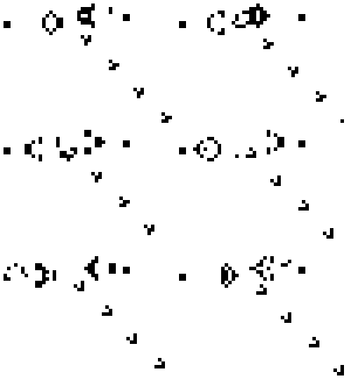
Cellular automata were introduced by Stanislaw Ulam in Los Alamos around 1940 . John von Neumann , a colleague of Ulam at the time, took up the idea and expanded it into a universal calculation model. He presented a cellular automaton with 29 states that could reproduce a given pattern again and again. He was the first to describe a cellular automaton that is universal in terms of calculation and design. According to von Neumann, it is suitable for problems of biological organization, self-reproduction and the evolution of complexity. The cellular automat is thus also an important basis for artificial life .
Up to the 1960s, which were analog computers to digital computers superior to some questions. An analog cellular automaton for simulation of groundwater flow is described in the article analog computer accurately.
In the 1970s, John Horton Conway's Game of Life became famous.
In 1969 Konrad Zuse published his book “Computing Space”, in which he assumes that the laws of nature follow discrete rules and that everything that happens in the universe is the result of the work of a gigantic cellular automaton.
In 1983 Stephen Wolfram published a series of foundational papers on cellular automata and in 2002 the book A New Kind of Science .
Wolfram's one-dimensional universe
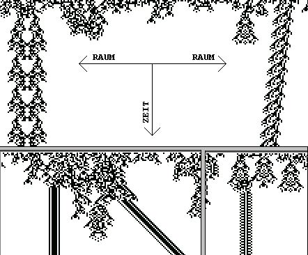
Computer scientist Stephen Wolframs cellular automaton is a particularly beautiful and simple model universe . It consists of only one space and one time dimension. In the picture the space dimension is drawn horizontally and the time dimension runs vertically downwards. (The picture contains three different sections of the picture.) The spatial dimension is finite, but unlimited, because its right and left ends are topologically connected.
The space-time elements of this universe can only be empty or full. In the case of the “ Big Bang ” (in the uppermost picture lines) these space-time elements are filled with a 50 percent probability. There is only one law of nature that represents a close-up effect. The near area comprises the left two neighbors of a space-time element, the space-time element itself, and the right two neighbors of the space-time element. If two or four space-time elements are full in the vicinity, then this space-time element is also full in the next time interval, otherwise it is empty in the next time interval. There are no other rules.
Although, in contrast to computer games, there is no action at a distance and no control authority whatsoever, this model universe is developing into astonishing complexity. After the Big Bang, there is an elimination phase, just like in the real universe. After that, short-lived but orderly structures emerge, which at some point disappear. However, some of the ordered structures are long-term stable, some of them oscillate, others are dimensionally stable over time. Both the oscillating and the dimensionally stable structures exist in both stationary and movable types. The maximum exchange speed of this universe can only be two units of space per unit of time. When collisions occur between the stable moving objects, chaos sets in again and another phase of elimination takes place.
If one simplifies even further and only takes into account the state of the element itself, only the right and left neighboring elements, there are exactly 8 rule elements. An example is given below. There are a total of 256 such rules. Even among these even simpler rules, some show astonishing complexity. One of the most interesting is the "rule 110":
Rule 110
| new state of the middle cell | 0 | 1 | 1 | 0 | 1 | 1 | 1 | 0 |
| current state of three neighboring cells | 111 | 110 | 101 | 100 | 011 | 010 | 001 | 000 |
See also: rule 30
Classification
In A New Kind of Science and in a number of papers from the mid-1980s, Stephen Wolfram defines four classes into which cellular automata (more precisely: the rules they work through) can be divided according to their behavior. Previous authors simply tried to identify the type of pattern for certain regulations.
According to the effort, these were the classes:
- Class 1: Almost all original patterns quickly develop into a stable and homogeneous state. As a result, any randomness in the first patterns disappears.
- Class 2: Almost all original patterns develop quickly into stable or oscillating structures. Some coincidences of the first patterns can be filtered out, but some can remain behind. Local changes to the original pattern tend to remain local.
- Class 3: Almost all of the original patterns develop in a pseudo-random or chaotic manner. Any stable structure can be quickly destroyed by noise. Local changes to the original pattern tend to spread to infinity.
- Class 4: Almost all original patterns develop into structures that interact in a complex and interesting manner. Finally, informative original patterns can, as is usual in class 2, result in stable or oscillating structures, but the number of steps required to achieve this state can be very large, even for simple patterns. Local changes to the original pattern can spread indefinitely.
Wolfram suggested that not all class 4 cellular automata are capable of performing universal computations. The universality has been confirmed especially for Rule 110 and Conway's Game of Life .
Programming cellular automata
This short script, written in the programming language Python , can simulate all 256 one-dimensional cellular automata and generates an image in the graphic format Portable Graymap (.pgm) as output . When calling up, the desired rule number, 0 to 255, must be entered.
 1 from optparse import OptionParser
 2
 3 if __name__=="__main__":
 4     parser = OptionParser()
 5     parser.add_option("-r", dest="rule", help="Rule number 0..255.")
 6     parser.add_option("-f", dest="file_path", help="File path")
 7
 8     (option, args) = parser.parse_args()
 9     rule = option.rule
10     file_path = option.file_path
11
12     w = 1000
13     r = s = [0] * w
14     r[int(w/2)] = 1
15     z = []
16     d = 0
17
18     for j in range(0, int(w/2)):
19         n = (r[0] << 1) + r[1]
20         o = ""
21         for i in range(1, w):
22             o += " 0 " if r[i]==1 else "15 "
23         z.append(o + "\n")
24         for i in range(2,w):
25             n = (n << 1) + r[i]
26             if n >= 8: n-=8
27             s[i-1] = (int(rule) >> n)%2
28         r = s
29         d += 1
30
31     f = open(file_path,'w')
32     f.write("P2\n")
33     f.write(str(w-1) + " " + str(d) + "\n")
34     f.write("15\n")
35     for i in range(len(z)-1, 0, -1):
36         f.write(z[i])
37     f.close()
Examples of cellular automata
- Conway's Game of Life is a simple two-dimensional cellular automaton that creates amazing structures.
- Langton loops simulate self-replicating organisms in a cellular automaton.
- The Pascal's triangle can also be interpreted as a simple cellular automaton.
- The Nagel-Schreckenberg model is a cellular machine for simulating road traffic , especially on motorways .
- The FHP model is used to simulate gases and liquids .
- A very simple cellular automaton is the ASEP .
See also
- Ant (Turing machine)
- Emergence
- Evacuation simulation
- Artificial life
- Pattern formation
- Predator prey model
- Turing machine
- Wator
- Wireworld
- Pascal's triangle can be simulated with cellular automata
- Finite automaton
literature
- Melanie Mitchell: Complexity. A guided tour. Oxford University Press, Oxford et al. 2009, ISBN 978-0-19-512441-5 , limited preview in Google Book Search.
- Klaus Mainzer , Leon Chua : The Universe as Automaton. From Simplicity and Symmetry to Complexity. Springer, Heidelberg et al. 2012, ISBN 978-3-642-23476-7 , limited preview in the Google book search.
Web links
Secondary literature
- Francesco Berto, Jacopo Tagliabue: Cellular Automata. In: Edward N. Zalta (Ed.): Stanford Encyclopedia of Philosophy .
- Jürgen Schmidhuber: Website about Konrad Zuse's theory of computing space ( extract from Electronic Data Processing 8 (1967) pp. 336–344)
Visualizations and implementations
- Wolfram's 1-dimensional universe as a C # implementation
- 2.5d cellular machine (3d game of life) with documentation and source code
- Greenberg-Hastings automata ( memento from June 18, 2010 in the Internet Archive ) as a Java applet
- Cyclic cellular automaton as Java applet
- Zellomat3D - 3D cellular automat
- NetLogo - agent-based modeling and simulation environment
- Random Design - Randomly generated cellular automata
- Order process in a Monte Carlo-based cellular automat (Youtube video)
- Otomata - Sequencer as an interactive cellular automaton
- Cafun - Freeware Java implementation for the simulation and visualization of cellular machines with XML-based configuration
- Golly - Simulation of numerous different cellular automata with examples
Individual evidence
- ^ Daniel Dennett, (1995), Darwin's Dangerous Idea, Penguin Books, London, ISBN 978-0-14-016734-4 , ISBN 0-14-016734-X
- ↑ NetLogo Models Library: CA 1D Elementary Cellular Automata. Accessed November 26, 2018 .


