Analog computer

Simulation of the drive train of a farm tractor with hybrid computer EAI-8800 and hardware-in-the-loop (1987)

Analog computers are computing devices or calculating machines with which calculations are carried out with the help of continuous mechanical or electrical processes. They differ from digital computers in that no pieces or events are counted and both the calculated values and the course of time are continuously mapped. In the slide rule , a simple mechanical analog computer, numbers are represented as continuously selectable lengths and the multiplication or division of numbers is mapped to a logarithmic addition or subtraction.

Analog computers take advantage of the property that there is a connection between the behavior of the original and the model in a certain area of validity ("principle of analogy"). The model can be used to simulate the behavior of the original , because the original and the model behave similarly (lat. "Simul") in the area of interest. Analog computers were initially used for specific technical relationships, for example to calculate control processes with the help of pneumatic or electrical equivalent circuits that mimicked the dynamic behavior. Another example was the mechanical tide calculator . From the 1940s on, analog computers were built on the basis of electron tubes and later transistors and operational amplifiers and standardized for general problem solving.

From the mid-1980s onwards, analog computers were increasingly replaced by digital computers, which became more and more powerful and inexpensive. In a transition period there were hybrid computers with a combination of analog and digital computers.

An analog computer : the slide rule

Compared to digital computers

Analog computers do not represent their data as discrete values like digital computers , but as continuous - just analog - quantities, for example in the form of geometric lengths, angles, water levels ( water integrator ), electrical voltages or currents. The equations are described in an electronic analog computer by wiring standardized components, in a digital computer by the program.

The great advantage of analog computers compared to digital computers is their real-time capability and their high parallelism due to the principle involved, up to the frequency range of 20 kHz . Compared to algorithmically programmed machines, this leads to a significantly greater computing power with, however, less computational accuracy, which in the best case is around 0.01 percent.

History of the analog computer

Antikythera Mechanism

Well-known old examples of analog computers are the various types of slide rules and mechanical planimeters that were widely used from the 19th century until they were replaced by digital electronic devices in the 1970s and 1980s. Proportional angles, reduction circles and (for drawing) pantographs and coordinateographs were also widely used. Slide rules were mainly available in the forms of slide rules, slide rules, slide rules and calculating clocks.

The oldest known device with an analog function is the Antikythera Mechanism , which dates back to around 150 BC. Is dated. With it, lunar and solar eclipses as well as the Olympics could be determined. The Antikythera mechanism only represented fixed, pre-factorized relationships between several periodically variable quantities, so it was not actually calculated.

To calculate tides , mechanical analog computers were used, as can be seen in the German Maritime Museum in Bremerhaven or in Wilhelmshaven . Mechanical gears served as integrators that were coupled with one another via pulley gears in order to simulate the influence of the moon, the sun and the rotation of the earth as well as some other parameters.

In 1919 Vannevar Bush worked as a scientist at MIT, and from 1923 as a professor of electrical engineering. There he developed an analog computer for solving differential equations , the Product Integraph, between 1923 and 1927 . The Differential Analyzer was an electromechanical analog computer that could integrate several differential equations at the same time. The output took place by means of automatically printed diagrams. It was developed from 1928 to 1932 at the Massachusetts Institute of Technology (MIT) under the direction of Vannevar Bush and H. L. Hazen.

The water integrator was built in 1936 in the Soviet Union. Analog dynamic calculations could be carried out using a complex network of pipes and water tanks .

During the Second World War, Sergei Alexejewitsch Lebedew worked on automatic controls for complex systems. His group developed an aiming device for tanks and a navigation system for missiles. To this end, he developed an analog computer for solving differential equations until 1945. At the same time, Hendrik Wade Bode in the USA developed a feedback automatic control system for anti-aircraft guns (Director T-10) based on radar data .

Helmut Hölzer (1912–1996) was a German engineer (TH Darmstadt, today TU Darmstadt ) who developed an electrical analog computer for stabilizing and steering the A4 ballistic missile at the Peenemünde Army Research Institute. The accelerations and directions measured with gyroscopes were integrated into distances and angles in a mixer . Thus were thruster and the internal circuit according to the predetermined desired course of the trajectory controlled.

Johannes Hoch (1913–1950) was a mechanical engineer ( University of Göttingen ) who further developed the mixer after the Ossawakim campaign in the Soviet Union and also created a computer for the orbit model with which the trajectory of a rocket could be calculated taking into account the variable coefficients . Together with the mixer, it made it possible to simulate the control system including the rowing machines before take-off.

Electronic analog computers

Electronic analog computers were developed and standardized between 1950 and 1980 for the standardized solution of linear and non-linear differential equations. Electronic analog computers were technically usable, for example, to simulate the trajectories of artillery shells and bombs , to investigate issues in reactor physics , in aerospace engineering, but also in mathematics , the simulation of processes , in optimization, etc.

The main element of a conventional electronic analog computer is the operational amplifier , which serves as the basis for the following active basic elements:

Totalizer (with multiple inputs)
Integrator (with the ability to temporarily stop integration)
Multiplier and Divider

In addition to these basic elements, electronic analog computers have coefficient potentiometers as input units that are used as voltage dividers to map variable coefficients . Function generators based on diode networks can be used to set non-linear characteristics. In addition, a large number of specialized accessories have been developed over the years. These include resolvers for converting between Cartesian coordinates and polar coordinates , delay elements for simulating signal delay times, noise generators for generating stochastic signals, and many more.

Oscilloscopes or line recorders are mostly used to display the results of a calculation . Here, the possibility of an analog computer to allow calculations to run faster or slower than in reality through time scaling comes into play. For example, it is possible to run the simulation of a simple ecosystem with extremely increased speed, while other processes, which in reality run too quickly for a direct investigation (reaction kinetic questions in chemistry, etc.), can be investigated more slowly. By (manually) adjusting coefficient parameters, the result can be interactively varied or optimized in a simple manner.

In addition to the limited computational accuracy, there is the additional problem with electronic analog computers of a value range limited to a so-called machine unit. When using electron tubes , the machine unit was mostly 100 V, while, with a few exceptions, transistorized analog computers mostly worked with 10 V as machine unit. Exceeding this value range in the course of a calculation led to an overload and triggered an alarm on the computer. The differential equations must be modified by suitable scaling in such a way that, on the one hand, there is no overdriving in their solution, but on the other hand, the value range of +/- 1 machine unit is always as good as possible in order to keep calculation errors low. In this regard, an analog electronic computer can be compared with a certain right to a digital fixed point system, which has similar restrictions on the range of values. In the 1970s, transistor-based analog computers could achieve an accuracy of 4 decimal places with reasonable effort. In most cases this was more than sufficient, since the parameters of the simulated model could only be determined much less precisely.

Most of the commercially available analog computers had a central socket field (patch field) on which the respective computing circuits to solve a problem were set up with the help of plug connections (shielded cables were used in precision computers). Switching from one circuit to the next required replacing a switchboard (with the socket panel) and setting the coefficient potentiometer accordingly, so that a comparatively quick switch between problems was possible.

Examples of analog computer systems

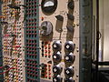
Analog computer programming via patch panel and potentiometer (Boeing, 1953)

AKAT-1 electronic analog computer from Jacek Karpiński in Poland (1959)

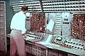
Newmark electronic analog computer (1960)

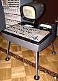
PACE 231R analog computer for simulating the X-15 experimental aircraft

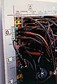
Circuit board of the hybrid computer EAI-8800 for simulating a wheel-rail system (1985)

Circuit board of the hybrid computer EAI-8800 (rear view of the contact level)

Example: Cellular Automat

Analog circuit for a maze

Analog circuit for groundwater

In the early days of the development of electronic analog computers, there were attempts to address problems by forming direct analogies with the help of mainly passive elements such as resistors, capacitors and coils.

The paths through a maze can be modeled with a network of resistances according to the respective partial length of a section. If you apply a voltage between the input and the output, you can find the shortest route by taking the direction with the greatest current flow at each fork. The basic principle of the solution is based on the distribution of current through a resistor network with parallel and serial elements. Similarly, a stream of water would find the fastest route through the maze, provided there was a steady gradient between the entrance and the exit.

The construction of an analog cellular machine for the simulation of groundwater currents with underground reservoirs is more functional. A two-dimensional field of capacitors was put together, the capacity of which corresponded to the water storage capacity of a small part of the soil, and these were then connected to their direct neighbors with resistors , the conductivity of the resistances corresponding to the water permeability of the corresponding part of the soil. In addition, there were now source areas as voltage introductions controlled by resistors , and wells as voltage discharges controlled by resistors. The voltage of the capacitor measured at the nodes of this network (i.e. the integral of the sum of all charging currents) then corresponded to the expected groundwater level , and the currents in the resistors corresponded to the expected groundwater flow.

Example: Equation of oscillation of a spring pendulum

Analog computing circuit for simulating a spring pendulum (without scaling to machine units)

The main area of application of analog computers is solving differential equations . An oscillation equation is a differential equation of the second order, as described, for example, for a spring pendulum by . Here is the vertical displacement of a mass , the damping constant , the spring constant and the acceleration due to gravity . For the analog computer, the equation is solved and thus receives the form . The corresponding calculation circuit requires two integrators with the state variables for the velocity or for the position of the mass, an adder for inverting on and three potentiometers for the coefficients. These components are connected by a total of eight plug-in cables. It should be noted here that the integrators and summers of an analog computer invert the input signals just like operational amplifiers. ${\ displaystyle m {\ ddot {y}} + d {\ dot {y}} + cy = mg}$ ${\ displaystyle y}$ ${\ displaystyle m}$ ${\ displaystyle d}$ ${\ displaystyle c}$ ${\ displaystyle g}$ ${\ displaystyle {\ ddot {y}}}$ ${\ displaystyle {\ ddot {y}} = - {\ tfrac {d} {m}} {\ dot {y}} - {\ tfrac {c} {m}} yg}$ ${\ displaystyle - {\ dot {y}}}$ ${\ displaystyle y}$ ${\ displaystyle y}$ ${\ displaystyle -y}$

The necessary scalings to machine units result intuitively from the order of magnitude of the physical state variables (in the physical units or ) or from the quotients of the coefficients in connection with selectable input gains of the integrators (typically 1, 10, 100). The solution results in a linearly damped oscillation with a stable end position due to earthly gravity and the spring constant. ${\ displaystyle m}$ ${\ displaystyle {\ tfrac {m} {s}}}$ ${\ displaystyle y = {\ tfrac {m} {c}} g}$

Example: Sinus run of a wheel-rail system

Animated representation of the sine curve

The dynamic behavior of a bogie in a wheel-rail system requires a complex non-linear simulation model. At higher speeds, the system tends to oscillate, the so-called sinusoidal run , and even, if it is insufficiently designed, to instability. The contact between the wheel and the rail is due to the profiling of the flange, which prevents derailment, non-linear and the degrees of freedom are coupled with each other. A railway wagon with two bogies has approx. 50 to 70 state variables and can therefore no longer be displayed even with the largest hybrid computer EAI-8800. Its simulation therefore requires the interconnection of several hybrid computers and the multiplexing of the forces on a wheel in order to determine the state variables of the wheelsets of a bogie. With the assigned digital computer, optimization calculations were carried out by varying the parameters of the hybrid simulation in order to achieve the most stable running behavior possible.

Hybrid computer

Towards the end of the 1960s, so-called hybrid computers were increasingly developed and used, which had digital and analog arithmetic units in order to combine the advantages of both technologies, the analog and the digital. This coupling enabled extended simulation options with complex maps or optimization methods with variation of parameters. The conversion between the types of representation with continuous (mostly electrical voltages) or numerical values was carried out with analog-digital or digital-analog converters .

Others

Modular synthesizers have the same structure as electronic analog computers. Famous manufacturers of mathematical instruments were Amsler (Schaffhausen), Coradi (Zurich) and Ott (Kempten). Integrating systems came from z. B. by Telefunken, Amsler and Contraves.

literature

Wolfgang Giloi , Rudolf Lauber: Analog computing . Springer, 1963.
Sigvard Strandh: The machine - history, elements, function . Herder, 1980, ISBN 3-451-18873-2 , pp. 191 .
Achim Sydow: programming technology for electronic analog computers . VEB Verlag Technik, 1964.
H. Adler, G. Neidhold: Electronic analog and hybrid computers . No. 206-435 / 197/74 . VEB Deutscher Verlag der Wissenschaften, Berlin (East) 1974.
Herbert Bruderer: Milestones in computer technology . Volume 1: Mechanical calculating machines, slide rules, historical automatons and scientific instruments, 2nd, strongly exp. Edition, Walter de Gruyter, Berlin / Boston 2018, ISBN 978-3-11-051827-6
Bernd Ulmann: Analog computers, marvels of technology - basics, history and application . 2010, ISBN 978-3-486-59203-0 .
James S. Small: The analogue alternative. The electronic analogue computer in Britain and the USA, 1930-1975 , Routledge 2001

Web links

Commons : Analog computers - collection of images, videos and audio files

The Analog Computer Museum Collection of electronic analog computers with extensive documentation for download as well as many practical examples.

Representation of a Joukowski profile with flow lines on an analog computer

Historical analog and hybrid computers with detailed images of their breadboards

Newer research project FACETS (Fast Analog Computing with Emergent Transient States)

Lecture by Bernd Ulmann at the Vintage Computing Festival Berlin (VCFB) 2015 about analog computer programming and the Easterhegg 2017 about analog computing

Individual evidence

^ Alfred Schmidt: What real-time simulation can do today (part 1) . Ed .: Electronics. No. 17/1992 . Franzis-Verlag, Munich, August 18, 1992, p. 52-57 .
^ First German tide calculator from 1914 in Wilhelmshaven
↑ Helmut Hoelzer's Fully Electronic Analog Computer used in the German V2 (A4) rockets. (PDF file; 497 kB)
↑ Boris Evsejewitsch Tschertok : Rockets and people. German missiles in Soviet hands . Elbe-Dnjepr-Verlag, Klitzschen 1998, ISBN 3-933395-00-3 , p. 251 f . (500 pages).
↑ System Description EAI-8800 Scientific Computing System. (PDF; 2.62 MB) Electronic Associates, Inc. (EAI), May 1, 1965, accessed September 5, 2019 .
↑ Alfred Schmidt; Lutz Mauer: Hybrid Simulation of the Nonlinear Dynamics of High-speed Railway Vehicles [1] , Springer-Verlag, 1988
^ Peter Meinke, A. Mielcarek: Design and Evaluation of Trucks for High-Speed Wheel / Rail Application . Ed .: International Center for Mechanical Sciences. tape 274 . Springer, Vienna 1982, p. 281-331 (English).

[1] Alfred Schmidt: What real-time simulation can do today (part 1) . Ed .: Electronics. No. 17/1992 . Franzis-Verlag, Munich, August 18, 1992, p. 52-57 .

[2] First German tide calculator from 1914 in Wilhelmshaven

[3] Helmut Hoelzer's Fully Electronic Analog Computer used in the German V2 (A4) rockets. (PDF file; 497 kB)

[4] Boris Evsejewitsch Tschertok : Rockets and people. German missiles in Soviet hands . Elbe-Dnjepr-Verlag, Klitzschen 1998, ISBN 3-933395-00-3 , p. 251 f . (500 pages).

[5] System Description EAI-8800 Scientific Computing System. (PDF; 2.62 MB) Electronic Associates, Inc. (EAI), May 1, 1965, accessed September 5, 2019 .

[6] Alfred Schmidt; Lutz Mauer: Hybrid Simulation of the Nonlinear Dynamics of High-speed Railway Vehicles [1] , Springer-Verlag, 1988

[7] Peter Meinke, A. Mielcarek: Design and Evaluation of Trucks for High-Speed Wheel / Rail Application . Ed .: International Center for Mechanical Sciences. tape 274 . Springer, Vienna 1982, p. 281-331 (English).