Slide rule

A simple slide rule. The tongue is set for a multiplication by 1.30, the position of the runner shows the result 2.60 for the factor 2.00.

Frank Whittle in practice

A slide or slide rule is an analog processing aids (also analog computer called) for the mechanical-graphical performing basic arithmetic operations , which preferably multiplication and division . Depending on the version, more complex arithmetic operations (including root , square , logarithm and trigonometric functions or parameterized conversions) can be carried out.

The principle of a slide rule is the graphical addition or subtraction of distances that are located as logarithmic scales on the fixed and moving parts of the slide rule. Until the widespread use of the pocket calculator , which began in the 1970s, slide rules were indispensable for many calculations in schools, science and technology.

The slide rule should not be confused with Napier's rulers , which make it easier to multiply two numbers by hand.

History of the slide rule at a glance

Logarithms: the mathematical basis

The history of the slide rule is based on the development of logarithms . Although there are Indian sources from the 2nd century BC. BC, in which logarithms for base 2 are already mentioned, it was the Swiss watchmaker Jost Bürgi (1558–1632) and the Scottish mathematician John Napier (1550–1617) who created the first known system for Developed logarithm calculation independently.

The Greek word "logarithm" means ratio in German and comes from Napier. Logarithms of this were first published in 1614 under the title Mirifici logarithmorum canonis descriptio, which can be translated as a description of the wonderful canon of logarithms .

After the Oxford professor Henry Briggs (1561-1630) dealt intensively with this font, he contacted the author and suggested using base 10 for the logarithms ("Briggs" or "decadic" logarithms). These spread quickly and were particularly valued in astronomy .

With the logarithms, the mathematical basis for the development of the mechanical slide rule was laid, because the mode of operation of the slide rule is based on the principle of addition and subtraction of logarithms for multiplication and division.

From logarithm to slide rule

As early as 1624, ten years after John Napier developed the concept of logarithms, the English theologian and mathematician Edmund Gunter (1581–1626) first announced his basic ideas about logarithmic numbers. With the "Gunters scale" he developed, a staff with logarithmically arranged scales, it was initially only possible to carry out multiplication and division calculations, including angular functions, with the help of a dividing circle by tapping the logarithmic lines. However, calculating with the compass was very time-consuming and labor-intensive. Richard Delamain published a circular slide rule with sliding scales in 1630, which he called Grammelogia. For the first time, it was possible to make calculations like a modern slide rule. William Oughtred (1574-1660) published in 1632 a disk rule with a set of fixed scales, which he called Circles of Proportions. The calculations were carried out with two pointers instead of the divider. In 1633, Oughtred published an addendum to the Circles of Proportions, in the appendix of which he describes the use of two mechanically disconnected rulers with logarithmic Gunters scales for arithmetic. Oughtred claimed to have invented his instruments, including a circular slide rule never published by him, before Delamain. Even if this were true, he did not publish his inventions; From his writings, in which he calls Delamain, among other things, a sleight of hand who impresses his students with the instruments, it is clear that his focus was on theoretical mathematics and not on mathematical instruments. Delamain must therefore be given the credit for having developed and described the slide rule for the public for the first time. Delamain was a student of Gunter ("Master Gunter, Professor of Astronomy at Gresham College, my worthy tutor"), so it is very likely, as Delamain claims, that Delamain's developments took place independently of Oughtred, even if Delamain and Oughtred knew each other and talked about mathematical questions. Edmund Wingates' arithmetic rulers had to continue to be used with compasses for dividing and multiplying; however, he first described today's scale combination D, A, K in 1645, so that it was possible for the first time to determine square and cubic roots without compasses and shifting the scale.

The first straight slide rule with a sliding tongue are known from Robert Bissaker (1654), and 1657 Seth Patridge (1603–1686). In Germany, logarithmic slide rules and rulers are only known about 50 years later, although calculators and rods were already known before 1630, but which probably worked on the basis of the relations in triangles and trigonometric functions.

The runner invented by Isaac Newton (1643–1727) - also known as the indicator - was implemented in 1775 by John Robertson (1712–1776). However, it was forgotten for over a hundred years. This extremely practical further development enables the connection of two non-touching scales with its cross-line marking and thus increases the accuracy of the tongue setting or reading.

The double logarithmic exponential scales to simplify exponential tasks of any kind were invented in 1815 by the English doctor and lexicographer Peter Mark Roget (1779–1869), only to be forgotten again by the beginning of the 20th century.

Until around 1800 slide rules were built in very different designs. In addition to the round slide rules and disks, in the center of which pointers could very easily be mounted, such as in Oughtred's Circles of Proportions, or a thread, as described by Delamain, a common elongated design consisted of a rod with a square cross-section and corresponding to the four sides with up to four tongues because there were no runners. These are derived from the rulers with mostly square cross-sections and scales on several sides, which were first described by Oughtred and which were placed next to each other in any combination and became known in Germany, for example, through the publication of Michael Scheffelt, who may have developed these independently himself .

The first slide rule to become more widespread is the type developed by James Watt , which is named Soho after his steam engine factory . This type became known in France and was produced there by Lenoir in high quality with engraved scales on boxwood. This type of slide rule only had one tongue and no runner either. Therefore, the upper scale on the body and tongue were plotted in two decades and used for multiplying and dividing. The lower scale on the tongue was also plotted in two decades and only the lower scale on the body was plotted in one decade; these two lower scales were used for root extraction and squaring. The back of the tongue of the Soho slide rule produced by Lenoir often also showed the sine, tangent and mantissa scales, whereby only the mantissa scale was related to the lower scale of the body.

From around 1850 the development of slide rules became extremely dynamic.

From everyday item to collector's item

In the first two hundred years after its invention, the slide rule was used very little. Only at the end of the 18th century was its importance newly recognized by James Watt .

With technical progress in the time of the Industrial Revolution , the slide rule became a widely used instrument for technical and scientific calculations. In the 1950 / 1960s it was considered the symbol of engineers, similar to the stethoscope for doctors. With the increasing importance of the slide rule, it was also taught in schools.

With the help of the slide rule not only locomotives, but also power plants, telephone networks and important structures such as the Golden Gate Bridge, as well as vehicles of all kinds, airplanes and missiles were constructed. Aluminum slide rules of the Pickett N600 type were also carried on Apollo space trips, including flights to the moon.

Every application of slide rules has special requirements, so that different types of slide rules have been developed. In addition to rather simple types, so-called school slide rules, which were used in lessons and for simple calculations in everyday life, more complex slide rules with various scale arrangements were designed for various technical tasks, so that engineers with different work focuses also used other slide rule types.

So-called special slide rules, some of which no longer allowed general calculations, were often used in very special areas, such as by pilots for navigation in aviation (as a calculating disc rule), in geodesy , electrical and systems engineering, chemistry , the military or in trade.

The first pocket calculators could only add and subtract in the early 1970s; therefore they were initially not a threat to the slide rule. As early as 1972, however, the HP-35 from Hewlett-Packard was the first technical and scientific pocket calculator with trigonometric, exponential and logarithmic functions. For a short time this gave a new impetus to the development of the slide rule; In 1970, the Aristo Hyperlog, probably the most sophisticated scientific slide rule made in Germany, came onto the market. However, by 1975 the prices for pocket calculators had fallen so far that school lessons were switched to them. With this, the slide rule finally lost its importance and production was discontinued. This happened around ten years later in the GDR and China. After that, slide rules were only used in a few areas, mostly in the form of special slide rules, for example for navigation in aviation, or for selecting heating valves.

Today, several decades after the end of the slide rule era, the slide rule is practically unknown to people younger than 50 years. However, a collector's scene developed which, beyond pure collecting, also played a major role in researching the history of slide rules. Meetings are held regularly in Germany and at the international level. The "Oughtred Society", which has existed since 1991, publishes specialist articles every quarter. There is also the international group "sliderule", which was previously on Yahoo .

Meanwhile there are also slide rule simulations and corresponding mobile phone apps, e.g. B. for the E6B flight computer. The graphical representation of slide rules is very well suited for operating concepts based on wiping, which is popular today.

Slide rule from 1850

The production of slide rules in large numbers and high quality started in France in the early 19th century by the company Lenoir and Gravet-Lenoir. Before the invention of the Mannheims type, they produced slide rules of the Soho type, which were used not only in England but also in France. From the end of the 19th century, the German companies Dennert and Pape, Faber-Castell and Nestler began to machine slide rules in large series.

Manufacturer overview

In the Federal Republic of Germany slide rules were z. B. von Aristo (Dennert & Pape) in Hamburg (from 1872 from Buchbaum, from 1888 with celluloid coverings), A. W. Faber Castell in Stein near Nuremberg (from approx. 1892), Nestler in Lahr (before 1900), IWA near Esslingen and at Ecobra produces. In the GDR it was the Reiss companies (later VEB Mess- und Zeichengerätebau) in Bad Liebenwerda and Meissner KG in Dresden. In 1974, both companies were merged to form VEB Mantissa in Dresden .

Well-known foreign manufacturers of slide rules were in the USA u. a. Keuffel & Esser (Hoboken), Dietzgen and Pickett. In Japan, slide rules were produced by Sun Hemmi, who also manufactured numerous slide rules for the American company Post, in France by Graphoplex and in Great Britain by Thornton, Unique and Blundell-Harling. In addition, there were numerous other lesser-known companies at home and abroad. The Swiss manufacturers of slide rules (various designs) include Loga, Billeter, National and Kern.

Designs

Basically, two designs can be distinguished: the one-sided model and the two-sided model. There are also special designs such as the calculating disc rule and the calculating roller.

One-sided model

The one-sided model consists of a closed body with a U-shaped cross-section on which several parallel scales are usually attached, a movable tongue with its own scales of the same type and a slide with a horizontal line marking that can be moved on the body . With some manufacturers, the U-shaped body is divided into two halves, which are connected with spring plates, celluloid or other parts in order to be able to adjust the flexibility of the tongue. Often the tongue and the body contain inlays in the form of metal, aluminum or iron bands, which should ensure dimensional accuracy and also allow straightening or bending of the tongue if it was warped. Despite these measures, there are today many single-sided slide rules whose tongue is slightly different in length than the body. This is mainly due to the fact that the tongue and body were not made from the same piece of wood in the closed construction.

Two-sided model

The two-sided model, often referred to as a duplex, consists of a two-part body , the two parts of which are connected by bars at the ends. The bars are either firmly glued or screwed and riveted. The movable tongue runs between the two halves of the body, the speed of which can be regulated when the bars are screwed and riveted. The tongue and body were made from the same sheet of raw material. Differences in length are therefore less common in the duplex model. Wooden duplex models without glued layers, however, tend to warp in the transverse profile, so that the runner sometimes jams in pre-war models. The runner , which can be moved on the body, has at least one hairline on both sides of the body. The hairlines are adjusted to each other so that not only scales on one side, but also scales on the front and back can be related to each other.

materials

The slide rules were originally mainly made of wood on which the scales were engraved. Occasionally, glued-on printed paper strips were also used, which had the advantage of being easier to read. From the end of the 19th century, white celluloid strips were glued onto the wood, on which the scales were engraved and filled with color, so that, like paper, it was very easy to read. Instead of wood, bamboo was also used as a carrier material in Asia. The wooden and bamboo slide rules were finally largely replaced by plastic models, preferably made of PVC. Some manufacturers also rely on printed or engraved aluminum. Brass and ivory are rarely found.

Overall lengths

The standard scale length - measured from the "1" to the "10" mark - of the slide rule models is 25 cm; small versions (e.g. pocket models) have a scale length of 12.5 cm, office or table models of 50 cm. Longer designs for even more precise calculations are also known. Demonstration models for use in schools and universities were often 1.8 m in length.

Special designs

Wrist watch ( pilot's chronograph ) with slide rule on the outside of the dial.

Variants of the slide rule are

1. the calculating disc rule , d. H. a slide rule, which is not designed as a straight rod, but circular, can also be found on the back of some parking discs and even on clocks, and
2. the calculating roller , d. H. a slide rule, the scales of which are arranged cylindrically divided into many (typically a few dozen) parts, whereby a greater effective scale length (typically a few meters) and thus a higher accuracy is achieved. Calculating rollers came onto the market in larger numbers from the second half of the 19th century. The largest calculating rollers (from Loga, Uster / Zurich) have a scale length of 24 m. Calculator clocks are another design.

Since you cannot add and subtract directly with the slide rule, there are versions for these two arithmetic operations that have a number slide (pen adder) on the back .

The history of the scale systems of single-sided slide rules

Scale systems describe which scales a slide rule has, to which other scales they are related and how the scales are arranged on the slide rule. The calculations possible with a slide rule differ depending on the existence, reference and arrangement of the scales. The following is the history of the scale arrangements for technical slide rules in large-scale production from 1900 onwards. An important source for this is the book "The Slide Rule: A Practical Manual" by Charles Newton Pickworth , which appeared in a total of 24 editions, and thus depicts the history of the single-sided slide rule, especially in England and Germany from 1900 to 1950.

Mannheim system

The French mathematics professor Amédée Mannheim (1831–1906) developed a selection and arrangement of scales for slide rules around 1850, which was widely and manufacturer-independent and shaped the slide rule market until the Second World War. In addition to the basic scales C and D, there were only square scales A and B on the front. With the Mannheim system, the runner was also introduced in order to be able to relate scales A and B as well as C and D to one another. The back of the tongue usually had a mantissa (for logarithms, related to D), a sine (related to A) and a tangent scale (related to D). Mostly there were cutouts on the back of the stick for reading these scales; the logarithmic scale was therefore usually shown inversely (in reverse order). The tongue could also be turned to use the sine and tangent scales; this saved time when many calculations had to be performed with trigonometric functions. Later Mannheim models were equipped with a reciprocal scale (inverse basic scale CI) on the front of the tongue.

System Beghin

The Beghin system was successfully launched on the French market around 1898 and was also known there under the name règle des écoles. It is characterized by the fact that, instead of the square scales A and B, it has two staggered or folded scales, which allow you to calculate quickly without pushing through or kicking the tongue and almost any mixing of the scales. It was originally developed around 1882 by Professor Tscherpaschinski from St. Petersburg, who ordered a prototype from the French manufacturer Tavernier-Gravet. The B scale was usually placed on the back of the tongue; sometimes the A scale is found above the folded scales. The mantissa scale L can be found on the front narrow side, or on the back of the tongue. Due to the lack of scale A at the usual point, both the tangent scale T and the sine scale S had to be related to the scale D. These slide rules also show the inverse scale CI very early on. Late versions such as the Graphoplex 660 have the L mantissa scale on the front of the tongue and the ST scale on the back of the tongue. The folded scales later became the trademark for all modern slide rules, especially the duplex models; Although the more modern slide rules are dominated by folding um , the late Chinese slide rules of the Flying Fish 1002, 1003 and 1200 types return to folding um . ${\displaystyle {\sqrt {10}}}$ ${\displaystyle \pi }$ ${\displaystyle {\sqrt {10}}}$

A special variant are so-called precision slide rules, which also have folded scales but are cut off at half the length so that the unfolded scales range from 1 to and the folded scales from to 10. In this case it is not possible to calculate faster with these scales, but with greater accuracy than with a slide rule of the same length, whose scales have the full length. ${\displaystyle {\sqrt {10}}}$ ${\displaystyle {\sqrt {10}}}$ ${\displaystyle {\sqrt {10}}}$

System Rietz

In 1902, the German engineer Max Rietz (1872–1956) added the cube scale K and the mantissa scale L to the front of the slide rule. As with the Beghin system, the sine scale was related to the D scale very early in the Rietz type slide rules. As a result, the range between 35 minutes and 5.6 degrees has been omitted; This area has been included in a new ST scale in the Rietz system. This arrangement of the trigonometric functions on the tongue has established itself internationally. A reciprocal scale was added later on the front of the tongue. The Rietz system was produced by all manufacturers from the 1920s and developed into one of the most widespread scale arrangements by the end of slide rule production. This arrangement was particularly popular for pocket models with a scale length of 12.5 cm. Some post-war models were called Rietz, although the scale arrangement does not match (e.g. Reiss Rietz Spezial).

System Log-Log Simplex (electrical)

From the early 20th century, the double logarithmic scales were developed. These scales, also called log-log or exponential scales, not only allow the calculation of arbitrary, even non-integer, powers and roots, but also the calculation of arbitrary logarithms in a simpler way than so-called mantissa scales, which only apply to certain logarithms. In the Davis Log-Log Rule, the two exponential scales and inverse exponential scales were arranged on the two sides of a second tongue. In the Perry Rule, an exponential scale and an inverse exponential scale were placed on the body. In the Yatoga three exponential scales and three inverse exponential scales were already arranged on the body, as was later established in duplex models. Initially, however, the arrangement of the electric slide rule prevailed, which was the first from Faber-Castell to come onto the market around 1906 (model 368). From around 1925, most manufacturers' two scales LL2 and LL3 were usually based on the basic scales C / D and aligned with Euler's number e, which means that the natural logarithm can be read off directly. They were often arranged on the top of the bar at the top and bottom, analogous to the K and L scales of the Rietz type. Later they were often placed next to each other to simplify the transition between the scales. Since the scales LL0 and LL1 are not absolutely necessary for technical use, they have generally been left out due to the lack of space on one-sided slide rules. The remaining scales originally followed the Mannheim system (at Faber-Castell until production was discontinued); many other manufacturers switched to the Rietz system by the end of the 1950s at the latest (e.g. Aristo Elektro 915, Graphoplex 640 and others). The Graphoplex 640, developed by Prof. André Séjourné around 1950, has a second C-scale on the back of the tongue, so that when the tongue is turned all types of calculations are possible without having to turn the slide rule; it is only necessary to dispense with the CI and B scale.

System differential simplex

A fundamental disadvantage of the Mannheim, Rietz and Log-Log Simplex types is that either the slide rule or the tongue must be turned to use the trigonometric functions. With the latter, it is usually no longer possible to carry out normal multiplications and divisions, so that the tongue might have to be turned more often. Hubert Boardman filed a patent on September 29, 1932 (GB411090) which describes the differential scales TD and ITD for tangent and SD and ISD for sine as well as the differential scales Y and Z for the differential mapping of the LL1 scale. These scales take up very little space; the four trigonometric differential scales occupy a length of the standard division and are arranged on the tongue. The differential LL1 scales Y and Z need only 1 cm on the left edge of the slide rule with a graduation length of 25 cm and are arranged on the body directly above and below the tongue. With the Thornton 101 an otherwise Rietz compatible slide rule was produced, with the Thornton 121 an otherwise Log-Log Simplex compatible electric slide rule. Both of them had all the scales on the surface. The Thornton 131 also had the typical electric slide rule scales for efficiency and voltage drop under the tongue. In the UK these slide rules were widespread and can be found often used on ebay UK (as of June 2019).

System Darmstadt (Simplex)

Slide rule system Darmstadt

The invention of the Darmstadt system is attributed to the Institute for Practical Mathematics (IPM) at the TH Darmstadt under the direction of Alwin Walther and took place around 1934. The Darmstadt type is a further development based on the Rietz type with a heavily modified scale arrangement. For reasons of space, the ST scale is initially omitted and has been replaced by a mark ρ. Instead of the mantissa scale L, the new logarithmically plotted Pythagorean scale P was arranged on the front edge of the rod, which, if the sine is known, directly supplies the cosine and vice versa. The mantissa scale was moved to the rear narrow side. The sine and tangent scales were moved from the tongue to the front narrow side of the rod body; the slide rule no longer had to be turned completely for trigonometric calculations. With the plastic models, the sine, tangent and mantissa scales were placed on the surface of the body; The ST scale is also found on the later models. The exponential scales LL1, LL2 and LL3 were found on the back of the tongue (see also Davis Rule in the Log-Log Simplex system), so that any exponent and roots can be calculated with the Darmstadt. The calculation of any logarithms was possible by turning the tongue. The Darmstadt type was produced by several German manufacturers from the start; it was able to assert itself as the standard slide rule for the scientific field in Germany from the end of the 1930s to the mid-1950s. Its scale diagram was adopted for the trigonometric functions on the German and British duplex slide rules; it has not caught on internationally. The original Simplex variant also remained one of the best-selling systems in the German market based on the Rietz system until the end of the slide rule era and was also very popular as a pocket slide rule.

The history of the two-way slide rule systems

Early duplex

The so-called duplex slide rule was reinvented by William Cox in 1891 and a patent was applied for for the American manufacturer Keuffel and Esser (K&E), so that other manufacturers could only enter the production of duplex slide rules later. The first duplex slide rules were nevertheless manufactured in large series in Germany by Dennert and Pape, because K&E first had to set up their production in the USA. A well-known model manufactured for K&E in Germany around 1903 is the K & E4078, which only had four scales on the front and back, namely A [BC] D and A [BI CI] D. Other early models, already from US -american production, the K & E4061 with identical scale arrangement and the K & E4061-T with additional trigonometric scales (A [BSC] D and A [BI T CI] DL). These slide rules are Mannheim compatible; the S scale is related to A. Around 1908 the K & E4092 was developed, which was the first Log-Log Simplex compatible duplex slide rule, and from the beginning also included the LL1 scale. Its two sides show A [BSC] D and LL1 LL2 LL3 [BT CI] DL; Here too, the S Mannheim scale is compatible with A.

After the K&E Duplex patent expired, other manufacturers in the USA began to produce duplex slide rules (e.g. Dietzgen) or sell them (e.g. Post), including those from Japan from the Hemmi company. Although the range of slide rules has diversified, some families of scales that build on one another can be identified.

Trig and Decitrig

Trig and Decitrig denotes the presence of the trigonometric functions ST and ST, usually on the tongue. Trig means that the division is made by degrees, minutes and seconds, Decitrig denotes the decimal division of degrees. Until the 1930s, the sine scale was usually based on the A scale instead of the D. From the 1950s onwards, the DI scale was also often available.

speed

Speed ​​indicates the presence of the so-called folded scales DF CF and CIF. These shifted scales allow faster calculation, since tongue movements can be saved. Usually the scales were shifted by π. The scale transition from the standard scales to the folded scales is multiplied by π; this enabled calculation steps to be saved.

Log-log

These slide rules had the double logarithmic scales on the body. From the 1920s, a special inverse scale LL0 was added to the K&E 4092-3. The latter is related to the A scale and delivers the result from A in the range 1… 13 and the result in the range 13… 100 . All (Deci) trig and Speed ​​scales were also available on this model. From the late 1940s, the inverse double logarithmic scales LL01, LL02 and LL03 were recorded (e.g. Pickett Model 2, K&E 4081-3). At that time, the manufacturer Pickett set new standards for the number of scales with its closely printed duplex slide rules made of aluminum; In some Pickett models, the LL scales were not related to D, but rather to folded scales, as was the case with Model 2. If the inverse exponential scales were available, the hyperbolic functions could also be determined relatively easily, so that no slide rule of the vector type described below could be purchased had to. The LL0 for scale can be replaced with sufficient accuracy by the D scale, which is why it and the LL00 scale have often been omitted. ${\displaystyle e^{-0,1x}}$ ${\displaystyle e^{-0,01x}}$ ${\displaystyle e^{0,001x}}$

vector

Vector slide rules had additional scales for calculating hyperbolic functions. The first usable slide rule of this type was developed by Mendell Penco Weinbach, who registered a design copyright for it on March 7, 1928. This slide rule had, among other things, the scales Th, Sh1 and Sh2. What was remarkable about its scale arrangement was that the trigonometric functions were initially attached to the body, as was later the case with the Darmstadt system (K & E4093). From 1938 the trigonometric functions were transferred to the tongue and the hyperbolic functions to the body (K & E4083). Usually the scales of all the above types were also available with the exception of the inverse exponential scales.

Around 1929 Sadatoshi Betsumiya and Jisuke Miyazaki invented the non-logarithmic Pythagorean scales P (not identical to Darmstadt!) And Q to calculate the trigonometric functions. With the invention of the Gudermann Gd scale around 1931, it was possible to calculate the hyperbolic functions using the P and Q scales with just one additional scale. This scale system achieved a relatively wide distribution with the Hemmi 153 in Japan, and from around 1938 also in the USA and China.

Precision (roots and cube roots)

Slide rule from one of the last series: Faber-Castell Novo Duplex 2 / 83N

Some slide rule types, mostly of the log-log type, were equipped with the root scales R1 and R2 (German: W1 W2) on the body from the 1950s (e.g. Post Versalog), which allowed a more precise determination of the squares and roots. From this time on, duplex slide rules with the cube roots 3R1, 3R2 and 3R3 can also be found on the body (e.g. Pickett N3). With the Faber-Castell 2/83 there was also a slide rule that had root scales not only on the body (W1 and W2), but also on the tongue (W1 'and W2'), so that it was possible to multiply and divide with increased accuracy . With these slide rules, the scales A and B are often omitted (e.g. Post Versalog Version I and Faber-Castell 2/83). This worsened the implementation of multiplications and divisions with root expressions, because more settings and value transfers were required. Because of the value transfers, the accuracy of the root scales could not be used in many cases. With the further developed Faber-Castell 2 / 83N, the A and B scales have been taken up again; however, the clarity suffered from the fact that they could not be arranged directly on the cutting edge between the tongue and the body.

German and British Duplex Sonderweg

As in the rest of Europe, duplex slide rules were practically unknown in Germany before the end of the Second World War. The pioneer in Germany and thus also in Europe was the Aristo company, which launched the Aristo Studio in the early 1950s, probably the most successful duplex slide rule in Germany for academic technical use. He had the trigonometric functions including the Pythagorean scale P arranged on the body as in Darmstadt. This arrangement prevailed in Germany for duplex slide rules. The exponential scales were arranged as is customary internationally for the log-log type. The hyperbolic slide rules from the manufacturer Aristo (Hyperbolog and Hyperlog) followed the international standard of vector slide rules.

In Great Britain only Thornton produced a duplex slide rule in good quality and in larger quantities for academic use: the P221 as the successor to the PIC121, and then the AA010 Comprehensive with an identical scale arrangement. This scale arrangement was compatible with the Aristo Studio including the normal trigonometric functions on the body. In addition, it had the DI scale, the differential trigonometric functions on the tongue known from the PIC121, and, probably the first in Europe, the H1 scale, referred to there as Pt, which was also found on the Aristo Hyperlog from 1970 onwards.

Special slide rule

Play media file

The Aristo Schul-Commerz, in trade from 1954 to 1970

All slide rule types have been optimized for special applications, even if they only have general scales; an example of this is the cube scale K, which is usually not available on a pocket calculator, and which could also be dispensed with on the slide rule. In a broader sense, special slide rules are understood to mean those slide rules that allow general calculations, but whose additional scales map very special mathematical expressions (e.g. Stadia system). In most cases, the additional scales eliminate general scales (exception: type electric (simplex)). Special slide rules in the narrower sense are those slide rules that no longer allow general calculations, but can only be used for special tasks. In many cases the scales are designed in such a way that a numerical value cannot stand for several values, but for exactly one value in exactly one unit. Another characteristic are special scales that replace technical table books. A slide rule for chemists was brought out by Verlag Chemie in cooperation with Faber-Castell.

System Stadia (surveying technology)

The trigonometric functions play an important role in technical survey calculations . Corresponding slide rules not only have scales for the elementary functions sinα, cosα, tanα, but also for more complex functions such as cos² (α), sin (α) cos (α), 1 / tan (α / 2). As a rule, there are no scales for this, e.g. For example, the scales A and B on the Nestler Geometer 0280. Since in surveying, angles are often not counted in degrees but in gons with decimal subdivisions (90 ° = 100 gon), there are slide rules of this kind (e.g. "Aristo geodesic “) Also in gon version, so that the argument of all trigonometric functions must be set in gons.

Electric

Calculating rods of the Log-Log Simplex type were mostly referred to as electric; some, but not all, had special scales. Mostly these were the scales for calculating efficiency levels and the voltage drop of direct current in copper lines, which were arranged under the tongue to save space and were related to the scales A / B; Standard scales of the Log-Log Simplex system are not omitted. Electric slide rakes often had marks for the conductivity and specific gravity of copper and aluminum. A special form of Elektro is the Diwa 311 Elektro; this has the additional scales for efficiency and voltage drop, but is not of the Log-Log Simplex type, but of the Darmstadt (Simplex) type.

Slide rule - only for special tasks

There are also slide rules for other special applications, e.g. B. for the selection of bearings or V-belts in mechanical engineering.

• Examples of special slide rules
• 

  Selection of V-belts

• 

  Machine tools working parameters

• 

  Humidity indicators

• 

  Pipe network computer for air ducts, front side

• 

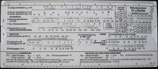
  Pipe network computer for air ducts, rear

functionality

introduction

With a few exceptions, it works based on the nature of the logarithm . Due to the logarithmic arrangement of the numbers, the properties of the logarithm can be used. The most important property is that the logarithm of the product of two numbers is the sum of the logarithms of both individual numbers:

${\displaystyle \lg(a\cdot b)=\lg(a)+\lg(b)}$

The multiplication of two numbers is transformed into a sum. In this way, multiplications can be carried out by adding lengths. Analog can about the relationship

${\displaystyle \lg \left({\frac {a}{b}}\right)=\lg(a)-\lg(b)}$

divisions can also be solved by subtracting distances.

Multiplication and division are carried out by adjusting the tongue and by means of carriage adjustments and value readings by adding and subtracting lengths. The runner allows different scales to be related to one another. Not only simple numbers can be multiplied and divided, but any function expressions that are stored in a scale; all logarithmic and double logarithmic scales can basically be combined with one another. The highest efficiency and the highest accuracy when using the slide rule is given when the number of tongue and slide movements and the number of value readings and transfers are minimal; the skillful combination is therefore essential.

Logarithmic scales in one and more decades

The scales of the slide rule have a certain total length L. This total length, also called the division length, is usually 125 mm for shirt pocket models, 250 mm for standard models and 500 mm for office models. Due to their limited length, the scales cannot accommodate the entire range of numbers. Usually only one or two decades are displayed. The numbers run from 1 to 10 for one decade (d = 1), or from 1 to 100 for two decades (d = 2). When using the logarithm of ten, this becomes one Number x associated length l (x) calculated as follows:

${\displaystyle l(x)={\frac {L}{d}}\cdot \lg(x)}$

Historically, two decades were initially used (scales A and B) because this made it easier to use the slide rule. Later, for reasons of accuracy, only one decade was used (scales C and D).

With a division length of 250 mm on scales A and B, the number 8 is 112.886 mm long. The product has the corresponding length . With two decades (* 2!) This length corresponds to the number . The result is obtained directly by adding the two distances. On scales C and D, the number 8 is 225.772 mm long. It is no longer possible to add the length of the two numbers because the total length is longer than the length of the division. Therefore, the so-called kickback must be applied. In the case of kickback, the division length is subtracted from the total length. This corresponds to division by 10. The product is thus calculated from the lengths ; this corresponds to the number 6.4. ${\displaystyle 8\cdot 8}$ ${\displaystyle 112,886\ \mathrm {mm} +112,886\ \mathrm {mm} =225,772\ \mathrm {mm} }$ ${\displaystyle 10^{\frac {225,772\cdot 2}{250}}=64}$ ${\displaystyle 8\cdot 8}$ ${\displaystyle 225,772\ \mathrm {mm} +225,772\ \mathrm {mm} -250\ \mathrm {mm} =201,544\ \mathrm {mm} }$

Many slide rule instructions therefore break down the calculation of the result into the determination of the sequence of digits and the determination of the location of the decimal point.

The basic scales in one and two decades allow the calculation of multiplication, division, reciprocal value as well as direct proportions such as the rule of three and the percentage calculation.

The transition from a scale in two decades to a scale in one decade corresponds to the square root of the number in question, and vice versa. Correspondingly, if the scale B exists, it can also be multiplied or divided directly with roots. For example, if the length of the number 2 on the scale B is added to the length of the number 2 on the scale D, the length of the number 2.83 results on the scale D. In other words, the result of can be calculated with a distance addition or a multiplication . Intermediate readings or value transfers are not required when different scales are combined. ${\displaystyle 2{\sqrt {2}}}$

The way in which graphical adding and subtracting works is initially independent of whether the result then appears on scale D or scale C or a scale on the body or a scale on the tongue. One function of the runner, however, is to temporarily store the results between two tongue movements, which is why it is usually most expedient if the result appears on a scale on the body, usually on the D and / or DF scale.

Calculation of the hypotenuse from the legs of a right triangle using only the base scales in one and two decades.

In some cases, however, it is also very elegant when intermediate results appear on a scale on the tongue. Little known is the solution of the right triangle by means of square scales, if the catheters, z. B. 3 cm and 4 cm, are known: The tongue is moved so that 1 on scale C is next to 3 on scale D. Then slide the runner onto 4 on scale D. Scale C now measures the length of . This corresponds to the tangent of the larger angle. Scale B measures accordingly at the point of the runner . The addition of 1 yields . If you set the length of this number to B by moving the cursor to 2.78, you read off the hypotenuse of 5 cm on C and D, which results from the length of 3 added to the length of . The end result is therefore advantageous again on the D scale. ${\displaystyle 4:3=1,33}$ ${\displaystyle \tan(\phi )}$ ${\displaystyle \tan ^{2}(\phi )=1,78}$ ${\displaystyle \tan ^{2}(\phi )+1=2,78=1/\cos ^{2}(\phi )}$ ${\displaystyle 1,66=1/\cos(\phi )}$ ${\displaystyle 1/\cos(\phi )}$

This example shows that in this case a division can advantageously be replaced by a multiplication with the reciprocal value. By skillfully using and coupling the scales in one and two decades, a comparatively complex task can be solved with just one tongue and two slider settings. In addition, the values ​​of the tangent, the cotangent (on the CI scale) and the cosine (on the CI scale) can be read without any further settings. Given the presence of the trigonometric scale T2 on the tongue, the angle would also be readable without further setting, in accordance with the mathematical relationships.

With the help of scale B and mental arithmetic, this example emulates a scale H on the tongue, which was not found on any German industrial slide rule. This scale is known on the Flying Fish 1002 and the Flying Fish 1003 from China; the scale H on the tongue saves adding 1 in the head. ${\displaystyle \tan ^{2}(\phi )+1}$

The cubic scale K in three decades is also often found in order to calculate or . ${\displaystyle x^{3}}$ ${\displaystyle {\sqrt[{3}]{x}}}$

Folded scales

Folded scales are only common in a decade to avoid the so-called kickback. Folded scales are calculated in the same way as the unfolded scales. The parameter f is the value by which the axis is shifted. Usually, it is postponed by, less often by and on commercial slide rules by for the commercial 360 days of the year. ${\displaystyle l(x)=L\cdot \lg(x-f)}$ ${\displaystyle \pi }$ ${\displaystyle {\sqrt {10}}}$ ${\displaystyle 3.6}$

The folded basic scales in a decade are usually used to calculate multiplication, division, and direct proportions such as the rule of three and the percentage calculation. The calculation results are independent of the parameter f, provided that two scales folded around the same parameter f, i.e. DF and CF or DF and CIF, are used. The index of CF always shows the same value on DF as the index from C to D, so that, in principle, you can continue to calculate on both the folded scales and the unfolded scales.

Folded scales can always be mixed with unfolded scales, but in this case you must read off the initial scale. Example : ${\displaystyle {\frac {1.5}{6}}}$

1. Runner on D 1.5
2. CF 6 on runner
3. Runner on CF 1, result on D

Since the index of CF is the same as the result, you can continue calculating immediately with the scales CF and CIF, whereby the result must be read off again on D.

Mixing up the scales can, however, lead to errors: When changing from a non-folded scale to a folded scale, it is multiplied by the parameter f and, conversely, divided by the parameter f. The convolution um can therefore also be used to calculate the multiplication with or the division by very efficiently by pure scale transition and without moving the tongue. ${\displaystyle \pi }$ ${\displaystyle \pi }$ ${\displaystyle \pi }$

Around folded scales: result on scales D and DF even when the folded and unfolded scales are mixed ${\displaystyle {\sqrt {10}}}$

The scales shifted by are a special case . With their help, the scale families can be mixed as desired. In the example above , the result can also be read on the DF scale if the index of C is used. Accordingly, you can continue to calculate directly with the scales C and CI if the result is then read off on DF. The reason for this is that when switching to the index of C, the factor is multiplied. With the transition to the folded scale, the factor is multiplied again so that it is multiplied by exactly . ${\displaystyle {\sqrt {10}}}$ ${\displaystyle 1,5/6}$ ${\displaystyle {\sqrt {10}}}$ ${\displaystyle {\sqrt {10}}}$ ${\displaystyle 10}$

This consideration also applies analogously to the transition from the DF scale to the D scale, in which case it is divided by. ${\displaystyle 10}$

Inverse scales

Inverse scales are labeled according to the formula . You run backwards with it. Until 1925, many slide rules did not have these scales; they managed to turn the tongue upside down. The inverse scales are commonly used to calculate multiplication, division, reciprocal values ​​and inverse proportions. By cleverly mixing the basic scale C and the inverse basic scale CI, series calculations can be carried out very efficiently. In addition to the inverse CI scale, the inverse folded scale CIF and the inverse double-decade scale BI are also common. ${\displaystyle l(x)=L\left(1-{\frac {\lg(x)}{d}}\right)}$

Function dials

introduction

Functional scales, such as the trigonometric scales, are determined according to the formula . The functions shown are not linear. For this reason, the labeling of the function scales only applies to the specific values. The basic scales assigned to the function scale, mostly C and D, rarely A and B, must also be interpreted in a certain range of values ​​for this function scale. Therefore, on some slide rules, next to the function scales, the factor or the value range with which the basic scales are to be interpreted is printed. ${\displaystyle l(x)=L\cdot \lg \left(f(x)\right)}$

Some function scales are therefore divided into several graduation lengths; for the tangent, for example, two pitch lengths with the scale designations T1 and T2 are common, which encompass the angles φ from 5.71 ° to 45 ° and 45 ° to 84.29 °. These correspond to the function values ​​tan (φ) from 0.1 to 1 and from 1 to 10.

The labeling of the function scales is not based on a uniform scheme. Certain abbreviations are usually used. In some cases the function shown is also indicated. Sometimes the function is specified, the x of which must be found on the function scale and whose function value can be found on the basic scales; sometimes it's the other way around. For this reason, for example, both the lettering and the lettering can be found for the double logarithmic scales . The factor with which the basic scales are to be interpreted is often given directly in the function value; For example, the function is written for LL2 , since the basic scale is to be interpreted in the range from 0.1 to 1. ${\displaystyle \ln(x)}$ ${\displaystyle e^{x}}$ ${\displaystyle e^{0,1x}}$

Functional scales can basically be used in two ways: First as a table, in which the function value is read on the basic scale C or D. The function scales can also be used as a factor. When arranged on the body, however, this is only possible for the first factor of a chain calculation. When placed on the tongue, the function scales can be used as any factors and divisors, which means that chain calculations that require several functions can be carried out more efficiently and more accurately because the values ​​do not have to be transferred.

Sine and tangent

The scale S (in), if it is related to the scales in a decade, is calculated according to the function , where x in a decade of the basic scales C and D - this corresponds to the division length - from the value range from 5.74 ° to 90 ° must come from. If you set a certain value on the C or D scale in the basic position of the tongue, strictly speaking, the S scale delivers the value where x is to be interpreted as C or D in the value range from 0.1 to 1. For smaller angles there is the ST scale, which runs for x on C or D between 0.01 and 0.1 from 0.573 ° to 5.73 ° and corresponds to a basic scale that is shifted by the fact that applies to small angles . The sine is represented in the range from 0.573 ° to 90 ° with two function scales, the value ranges of which differ and which have to be interpreted in the correct range on the basic scales. ${\displaystyle l(x)=L\cdot \lg \left(sin(x)\right)}$ ${\displaystyle \sin ^{-1}(x)}$ ${\displaystyle \pi /180}$ ${\displaystyle \sin(\phi )=\tan(\phi )=\pi \cdot \phi /180}$

The tangent is divided into up to four scales: the well-known ST scale, the T or T1 scale from 5.71 ° - 45 °, the value of which is to be interpreted from 0.1 to 1 in relation to C and D, the scale T2 from 45 ° to 84.29 °, where its value is to be interpreted in relation to C and D from 1 to 10, and rarely also the scale T3 from 84.29 ° to 89.427 °, where its value in relation to C and D should be interpreted from 10 to 100.

The cosine is usually labeled on the sine scale. Otherwise, it can easily be hired through the relationship . Ranges of values ​​that are not displayed on the scales must either be avoided by applying the rules of trigonometry or converted appropriately. ${\displaystyle \cos(\phi )=\sin(90-\phi )}$

The sin and tan scales can be used in exactly the same way as the basic scales, with the restriction that they are usually only on the body or on the tongue. If the scales are on the tongue (if necessary turn the tongue around!), The following example can be followed: The hypotenuse (5 cm) is known, as is the longer of the cathetus (4 cm). How long is the second leg? sin (90) corresponds to 1; if you put this at 5 on D, you read with the help of the cursor opposite from 4 on D 36.9 ° for the cosine (or 53.1 ° for the sine). It is calculated:, i.e. a division, the result of which appears on the tongue and is interpreted as a cosine and read off as an angle. Then push the slider further until the sin (36.9 °) is set. On D the result is 3 cm. It is counted as . This task can also be done with a tongue. and solve two slider settings, with the result appearing again advantageously on scale D and can be temporarily saved with the slider for the next tongue setting. ${\displaystyle \phi =\cos ^{-1}(4/5)}$ ${\displaystyle \sin(36,9)\cdot 5=3}$

The double logarithmic scales

The double logarithmic scales allow the calculation of arbitrary powers and logarithms.

According to the relationship , a power can be converted into a multiplication using a logarithm. This multiplication cannot yet be solved with a slide rule. Another logarithmization makes this possible: ${\displaystyle \log(a^{b})=b\cdot \log(a)}$

${\displaystyle \lg \left(\log(a^{b})\right)=\lg(b\cdot \log(a))=\lg(b)+\lg(\log(a))}$

Usually the natural logarithm is used for the inner logarithm, so that the so-called double logarithmic scales are calculated according to the formula . The double logarithmic scales thus represent a special case of the functional scales. ${\displaystyle l(x)=L\cdot \lg \left(ln(x)\right)}$

The double logarithmic scales are divided into up to four graduation lengths with the standard designations LL0, LL1, LL2 and LL3. The LL0 scale runs from 1.001 to 1.01 corresponding to the values ​​0.001 to 0.01 on the basic scale. The LL1 scale runs from 1.01 to 1.105 corresponding to the values ​​0.01 to 0.1 on the basic scales; LL2 runs from 1.105 to e corresponding to the values ​​0.1 to 1 and LL3 from e to 22000 corresponding to the values ​​1 to 10 on the basic scales.

The scale L3 is very imprecisely subdivided from the value 1000 at the latest, so that calculations can be carried out more precisely if it is divided into several factors. The division into factors can also be used for values ​​that exceed the range of values.

The double logarithmic scales are usually plotted symmetrically with the inverse double logarithmic scales on duplex models. The inverse double logarithmic scales are calculated using the formula . The ranges of these reciprocal scales LL00 to LL03 correspond to those of the scales LL0 to LL3 with regard to the basic scale values; the value ranges of the reciprocal scales LL00 to LL03 correspond exactly to the reciprocal values ​​of the scales LL0 to L L3. The symmetrical double logarithmic scales can therefore also be used very well to determine the reciprocal values, whereby the decimal point does not have to be determined yourself. ${\displaystyle l(x)=L\cdot \lg \left(ln(1/x)\right)}$

use

The scales

There are several (mostly logarithmic) scales on a stick or slide, each of which has a special function. The capital letters used in the table correspond to the usual designation on most modern slide rules. As a rule, each slide rule only has a selection of the listed scales. Since there are a large number of scale systems, the information about the position of the scale is not always generally valid. In addition, the individual systems are not always clear; the additional scales in particular were arranged differently by the individual manufacturers.

As a rule, the scales show values ​​increasing from left to right. Scales that decrease from left to right are usually labeled in red.

designation	Area	function	comment
A.	1 .. 100	${\displaystyle x^{2}{\mathrel {\widehat {=}}}D^{2}}$	Square scale for basic scale D on top of the rod body.
B.	1 .. 100	${\displaystyle x^{2}{\mathrel {\widehat {=}}}C^{2}}$	Square scale for basic scale C on the top of the tongue.
C.	1 .. 10	${\displaystyle \!\,x}$	Basic scale on the tongue.
CF	3 .. 1 .. 3	${\displaystyle \!\,\pi x}$	Basic scale C offset by π on top of tongue.
CI	10 .. 1	${\displaystyle x^{-1}{\mathrel {\widehat {=}}}C^{-1}}$	Reciprocal value of the basic scale C on the tongue.
CIF	0.3 .. 1 .. 0.3	${\displaystyle \!\,1/{\pi x}{\mathrel {\widehat {=}}}CF^{-1}}$	Reciprocal value of the basic scale C on the tongue, offset by π.
D.	1 .. 10	${\displaystyle \!\,x}$	Basic scale on the rod body.
DF	3 .. 1 .. 3	${\displaystyle \!\,\pi x}$	Basic scale D offset by π on the top of the rod body.
DI	10 .. 1	${\displaystyle x^{-1}{\mathrel {\widehat {=}}}D^{-1}}$	Reciprocal value of the basic scale D on the rod body.
DIF	0.3 .. 1 .. 0.3	${\displaystyle \!\,1/{\pi x}{\mathrel {\widehat {=}}}DF^{-1}}$	Reciprocal value of the basic scale D offset by π on the rod body.
K	1 .. 1000	${\displaystyle x^{3}{\mathrel {\widehat {=}}}D^{3}}$	Cubes or cubic scales (e.g. to determine a volume). Usually located on top of the rod body.
L.	[0], 0 .. [1], 0	${\displaystyle \log {x}{\mathrel {\widehat {=}}}\log {D}}$	Mantissa scale. Shows the mantissa of the decadal logarithm. The number must be determined independently. In contrast to the other scales, this scale is scaled linearly.
LL 1	1.010 .. 1.11	${\displaystyle \!\,e^{0{,}01x}}$	First exponential scale. In the Darmstadt type on the back of the tongue; in the case of the duplex type, at the bottom on the back of the rod body.
LL 2	1.10 .. 3.0	${\displaystyle \!\,e^{0{,}1x}}$	Second exponential scale. In the Darmstadt type on the back of the tongue; in the case of the duplex type, at the bottom on the back of the rod body.
LL 3	2.5 .. 5 · 10 4	${\displaystyle \!\,e^{x}}$	Third exponential scale. In the Darmstadt type on the back of the tongue; in the case of the duplex type, at the bottom on the back of the rod body.
LL 01	0.99 .. 0.9	${\displaystyle \!\,e^{-0{,}01x}}$	Reciprocal of LL 1 . In the case of the duplex type, at the top of the back of the rod body.
LL 02	1.91 .. 3.35	${\displaystyle \!\,e^{-0{,}1x}}$	Reciprocal of LL 2 . In the case of the duplex type, at the top of the back of the rod body.
LL 03	0.39 .. 2 · 10 −5	${\displaystyle \!\,e^{-x}}$	Reciprocal of LL 3 . In the case of the duplex type, at the top of the back of the rod body.
P	0.995 .. 0	${\displaystyle {\sqrt {1-(0{,}1x)^{2}}}}$	Pythagorean scale. With the Darmstadt and Duplex types at the bottom of the rod body.
S.	5.5 ° .. 90 °	${\displaystyle \sphericalangle \sin {0{,}1x}}$	Sine scale. Partly also with cosine scale in red letters. With the Rietz type, often on the back of the tongue.
ST	0.55 ° .. 5.5 °	${\displaystyle \sphericalangle \operatorname {arc} 0{,}01x}$	Radian scale for small angles. Also suitable for sine and tangent. With the Rietz type, often on the back of the tongue.
T or T 1	5.5 ° .. 45 °	${\displaystyle \sphericalangle \tan {0{,}1x}}$	Tangent scale for angles between 5.5 ° and 45 °. Partly also with cotangent scale in red letters. With the Rietz type, often on the back of the tongue.
T 2	45 ° .. 84.5 °	${\displaystyle \sphericalangle \tan {x}}$	Tangent scale for angles between 45 ° and 84.5 °. Partly also with cotangent scale in red letters.
W 1	1 .. 3.3	${\displaystyle {\sqrt {x}}}$	First fixed root scale. In the case of the Duplex type, at the bottom on the back of the rod body.
W 1 ′	1 .. 3.3	${\displaystyle {\sqrt {x}}}$	First movable root scale. For the Duplex type, at the bottom on the back of the tongue.
W 2	3 .. 10	${\displaystyle {\sqrt {10x}}}$	Second fixed root scale. In the case of the duplex type, at the top of the back of the rod body.
W 2 ′	3 .. 10	${\displaystyle {\sqrt {10x}}}$	Second movable root scale. For the Duplex type, on the top of the back of the tongue.

The runner

The movable runner is not only used for precise reading and setting of the various scales. It often also has additional runner lines that allow a simplified direct calculation. The short runner lines on the top left or bottom right are used in conjunction with the main line to calculate circular areas. Some models have additional markings for converting kW into PS or for direct calculation with a factor of 360 (e.g. for calculating interest).

Accuracy and decimal places

The accuracy with which a number can be set or read off depends on the size of the slide rule. With a 30 cm long slide rule, the numbers on the basic scales C and D can be set or read directly with an accuracy of two to three decimal places. One more decimal place can be estimated with a little practice. Larger slide rules have a finer subdivision of the scales and thus enable a more precise calculation.

Since the actual distances between numerically equidistant scale lines vary according to the logarithmic division, larger numbers can be set or read off with less precision than smaller numbers. The relative inaccuracy, i.e. the ratio of the inaccuracy of a number to the number itself, is the same for all numbers. Therefore, with several successive multiplications, not only the result but also its accuracy is independent of the order in which the individual multiplication steps are carried out.

However, the slide rule does not show the magnitude of a number. So z. B. the reading 6 and 6; 60; 600, but also 0.6; 0.06; Mean 0.006 etc. The position of the comma is determined by a rough calculation. This is essential for the correct use of the slide rule.

multiplication

Multiplication is the simplest and at the same time the most original type of calculation of the slide rule. It is based on the calculation rule that the logarithm of a product is equal to the sum of the logarithms of the individual factors.

Since the scales C and D are logarithmically divided on the slide rule, a sum of two logarithms is obtained by geometrically adding two distances on these scales. First, the starting mark “1” on the movable scale C (on the tongue) is pushed over the first factor on the fixed scale D. The runner is now pushed over the second factor on scale C. The result is read off the D scale at this point.

Example of the calculation ${\displaystyle 2\cdot 3=6}$

If the product exceeds the value 10, this cannot be read off in the manner described. Now imagine adding a virtual second D-scale to the end of the first. This corresponds to a shift of 10 on the C scale above the first factor on the D scale. The product can then be read off with the help of the runner under the second factor of the C scale on D. This procedure is called “pushing through” or “kicking back” the tongue.

Example of the calculation ${\displaystyle 2\cdot 5=10}$

Using the same method, you can use the scales A and B for multiplication. This is very useful when one of the factors is a square number, or when you want to get a square root from the product. This procedure is rather unusual for simple multiplication, as the greater division of the scales A and B results in less accuracy.

division

The Division is the inverse of multiplication. It is based on the calculation rule that the logarithm of a quotient (numerator divided by denominator) is equal to the difference between the logarithm of the dividend (numerator) and the logarithm of the divisor (denominator).

First the divisor on the movable scale C (on the tongue) is slid over the dividends on the fixed scale D. The runner is now pushed onto the starting mark “1” on the C scale. The result is read off the D scale at this point.

Example of the calculation ${\displaystyle {\frac {5{,}5}{2}}=2{,}75}$

If the quotient falls below the value 1, the result can alternatively be read from the end marking "10" on the movable scale C.

Example of the calculation ${\displaystyle {\frac {10}{5}}=2}$

Using the same method, the scales A and B can also be used for division; however, the accuracy is lower.

Another possibility is to multiply the dividend by the reciprocal of the divisor. Proceed in the same way as with multiplication, the only difference being that instead of the tongue scale C, the reciprocal value scale CI is used.

Proportions

The ratio between the values ​​on the scales C and D or A and B is always the same with the tongue setting unchanged.

Thus, the slide rule is very well suited for proportional calculations or for rule of three tasks . Here it is helpful to carry out the division before the multiplication, as the task can then usually be calculated with a single tongue setting.

A major advantage of the slide rule in the case of three rule calculations is that not only the result for the second factor, but also for any number of other factors can be read with the same tongue setting.

An example for creating a table: You want to convert English yards into meters and vice versa. The ratio is 82 yards are 75 meters. To do this, place the value 75 on the movable scale C above the value 82 on the fixed scale D. Now you can read the corresponding number of meters on the scale C for any values ​​of yards on the scale D. Conversely, for any number of meters on the C scale, the corresponding number of yards can be read off on the D scale.

Potencies

Square numbers

Example of square or cube number runner line on number: D # 2, result on scale A # 4 or K # 8

The relation applies to the square scales A and B.

${\displaystyle \log x^{2}=2\log x}$,

d. That is, they have two decades (1 to 10 and 10 to 100) in the range of the basic decade (1 to 10).

The squaring takes place through the transition from the scale C or D to the scale B or A, whereby the middle cursor line is advantageously used. One sets the runner line z. B. on the value on scale D and reads the square number on scale A.

With some slide rules there is a short additional line on the runner above the square scales A and B, which is offset by the distance π / 4. With the help of this additional line, the area of ​​the circle can be read off directly on scales A or B if the circle diameter is set with the middle line of the rotor on scales C or D.

Cube numbers

For the cube or cube scale K, the relationship applies

${\displaystyle \log x^{3}=3\log x}$,

d. That is, it has three decades (1 to 10, 10 to 100 and 100 to 1000) in the range of the basic decade.

The cubic number is determined by transitioning from scale D to scale K, with the middle runner line advantageously being used.

root

square root

In order to determine the square root of a number with a value between 1 and 100, you set this number with the runner on the scale A or B and read the result on the basic scale D or C.

If the square root of a number is to be determined whose value is not between 1 and 100, the radicand is divided into two factors, one factor being a power to the base 100 and the second factor being in the range between 1 and 100. According to the formula , you can take the root of each factor separately and multiply the results. ${\displaystyle {\sqrt {100^{a}\,x}}=10^{a}{\sqrt {x}}\,}$

The following rule of thumb can also be used: All numbers greater than 1 with an odd number of digits before the decimal point and all numbers less than 1 with an uneven number of zeros after the decimal point are set in the left decade (1 to 10) of scale A. All numbers greater than 1 with an even number of digits before the decimal point and all numbers less than 1 with an even number of zeros (also 0 is an even number) after the decimal point are set in the right decade (10 to 100) of scale A.

Cube root

In order to determine the cube root of a number with a value between 1 and 1000, you set this number with the cursor on the K scale and read the result on the basic scale D.

If the cube root of a number is to be determined, the value of which is not between 1 and 1000, the radicand is divided into two factors, one factor being a power to the base 1000 and the second factor being in the range between 1 and 1000. According to the formula , you can take the root of each factor separately and multiply the results. ${\displaystyle {\sqrt[{3}]{1000^{a}\,x}}=10^{a}{\sqrt[{3}]{x}}\,}$

Reciprocals

The reciprocal scales CI and DI correspond in appearance to the basic scales C and D, but run in the opposite direction. They are therefore mostly colored red. These scales can be used for various calculation options.

If the reciprocal value of a number is to be determined, this number is set on the basic scale with the cursor and the reciprocal value is read off directly on the reciprocal value scale.

With the help of the reciprocal scale, the calculation of a multiplication can be replaced by a division and vice versa. The following applies: A number is multiplied by dividing by the reciprocal value. This enables products from several factors to be identified with fewer tongue adjustments.

Compound multiplications and divisions can be calculated more efficiently with the reciprocal scales.

The reciprocal scales can also be used for trigonometric functions and exponential calculations.

Logarithm determination

The linearly divided logarithm or mantissa scale L contains values ​​for the mantissa (decimal places) of the decadic logarithm .

To determine the decadic logarithm of a number, set it on the basic scale D with the cursor and read the mantissa on the mantissa scale L. The key figure ( digit in front of the decimal point ) of the logarithm results, just as when using a logarithm table , for numbers greater than or equal to 1 from the number of digits before the decimal point minus 1. For numbers less than 1, the number of zeros after the decimal point is determined. This number is set negative and reduced by 1. As a rule of thumb, the following applies: The code corresponds to the number of places by which the comma must be shifted until there is exactly one digit other than zero in front of the comma. A shift to the left is assessed as positive, a shift to the right as negative.

The logarithm determination is mainly used to calculate powers and roots of any exponent. However, since even small inaccuracies when determining the logarithm significantly impair the final accuracy, this method is only used for rough calculations.

Trigonometric values

The following applies to all trigonometric functions: If an angle is given that is greater than 90 °, it must first be reduced to an acute angle that provides the same function value.

Sine

The sine scale S is subdivided decimally and, in conjunction with the basic scale D, gives the angle function or, if the reading is reversed, the angle.

The sine value for angles between 5.7 ° and 90 ° can be determined by setting the number of degrees on the sine scale S with the cursor and reading the function value on scale D.

Sine values ​​for angles smaller than 5.7 ° can be determined with the radian scale ST (see below).

cosine

The sine scale S is usually also labeled with red angle values ​​that increase from right to left. These values, in the interval from 0 ° to 84.3 °, represent the complement angle and enable the cosine value to be read on the basic scale D. Conversely, the associated angle can be determined.

tangent

The scales T1 and T2 are used to determine the tangent values, T1 being used for angle values ​​between 5.7 ° and 45 ° and T2 for angle values ​​between 45 ° and 84.3 °. The tangential value is read off on the basic scale D. Conversely, the corresponding angle can be determined.

The cotangent value can be read on the reciprocal value scale DI.

Tangent values ​​for angles smaller than 5.7 ° can be determined with the radian scale ST (see below).

For angle values ​​between 84.3 ° and 90 °, the complement angle is determined and set on the radian scale ST. After the relationship , the tangential value can be read off on the reciprocal value scale DI. ${\displaystyle \tan {x}=\cot {(90^{\circ }-x)}}$

Radians

The radian scale ST is subdivided in decimal and, in connection with the basic scale D, gives the radian or, if the reading is reversed, the angle.

The radian measure for angles between 0.57 ° and 5.7 ° can be determined by using the runner to set the number of degrees on the radian measure scale ST and read off the radian measure on the basic scale D.

The relationship applies to angles below 5.7 ° . This means that the radian measure roughly corresponds to the sine function and the tangent function. The deviation here is less than 1.5 ‰. This is why this scale is also used to determine sine and tangent values ​​for small angles. ${\displaystyle \mathrm {arc} \,x\approx \sin x\approx \tan x}$

General power calculations

The three exponential scales LL ₁ , LL ₂ , LL ₃ , lined up, represent the natural logarithm for the function values ​​1.01 to 50000. With the help of these scales any powers, roots and logarithms can be calculated. The exponential scales are place value scales; In other words, its decimal value corresponds to the inscription and cannot be changed as with the basic scales.

Addition and subtraction

An addition or subtraction is not directly possible with conventional slide rules. However, you can achieve your goal by transforming the addition problem into a multiplication problem.

A suitable formula is derived by excluding. It applies ${\displaystyle y}$

${\displaystyle x+y=\left({\frac {x}{y}}+1\right)\;y}$  for addition and

${\displaystyle x-y=\left({\frac {x}{y}}-1\right)\;y}$  for subtraction.

This task can be solved by using division and multiplication with the slide rule. The addition or subtraction of the number 1 required as an intermediate result can be done in the head. This type of calculation is certainly not trivial and hardly plays a role when using the slide rule.

In the case of slide rules with linear scales, the addition and subtraction can be carried out directly.

Clocks

There are still wristwatches that are equipped with a slide rule, for example from Breitling , Sinn , Casio or Citizen .

See also

• Abacus (arithmetic aid)
• Adding machine
• Calculating disc rule
• Logarithm table
• Nomogram

literature

• Herbert Bruderer: Milestones in computer technology. Volume 1: Mechanical calculating machines, slide rules, historical automatons and scientific instruments. 2nd, greatly expanded edition. Walter de Gruyter , Berlin / Boston 2018, ISBN 978-3-11-051827-6 .
• Ulla Fölsing: A hard line over the heart - an antique for today's students: the slide rule. An Altona exhibition about its history. In: Frankfurter Allgemeine Zeitung , Wednesday, June 22, 2011, No. 143, p. N5.
• Peter Hopp: Slide Rules: their history, models and makers. Astragal Press, Mendham 1999.
• Wilhelm Rieck: Rod Computing in Theory and Practice . Verlag Handwerk und Technik, 1971.
• Clifford Stoll : When computers were still being pushed (PDF; 530 kB) , Spectrum of Science , April 2007.

Web links

Commons : Slide rule  - collection of images, videos and audio files

Wiktionary: slide rule  - explanations of meanings, word origins, synonyms, translations

• Heinz Joss: History of the slide rule: everyday yesterday, forgotten today. In: Computer Lexicon - The Great Encyclopedia of Mechanical Computing, 2004.
• Overview of different types of slide rules
• Website of the University of Greifswald about different types of slide rules
• Slide rule letter. Site of the German-speaking slide rule collectors
• Slide rule online museum
• interactive online slide rule
• Slide rule programmed in PostScript

Individual evidence

1. ^ Richard Delamain: Grammelogia - or the mathematical ring, 1630
2. ^ William Oughtred: The Circles of Proportion, 1632
3. ^ William Oughtred: An addition onto the use of the instrument called the circles of proportions
4. ^ Richard Delamain: Grammelogia - or the mathematical ring, 1630; Preface
5. ^ Edmund Wingate: The Use of the Rule of Proportion in Arithmetick & Geometrie, 1645.
6. ↑ Hans Gaab: The engineer staff of 1650 by Trew , PDF
7. ↑ Michael Scheffelt: Pes mechanicus artificialis or newly invented measure rod, Ulm, 1718
8. ^ Rolf Jäger: Aristo novelties . In: Aristo (Hrsg.): Communications for engineering and universities . tape 12 . Hamburg January 1970, p. 15th f .
9. ↑ [e-mail]. Retrieved October 27, 2019 (American English). 
10. ↑ [e-mail]. Retrieved October 27, 2019 (American English). 
11. ↑ The slide rule REISS Duplex 3227 compared to other models. (Query date May 6, 2010; PDF; 2.6 MB).
12. ^ Cajori (1909): History of the logarithmic slide rule
13. ↑ Beghin slide rule with CI scale , accessed on August 6, 2019
14. ^ Règle à calcul. Retrieved June 7, 2019 . 
15. ↑ Rolf Jäger: The history of the slide rule . In: Notices for engineering and universities . No. 1 . Dennert & Pape, Hamburg September 1957, p. 3 .
16. ↑ Sphere's Auction Slide Rule Page - K + E's How to Pick a Slide Rule. Retrieved June 7, 2019 . 
17. ↑ | Slide rule for chemists
18. ↑ CASTELL slide rule textbook, Lindauer Verlag, 13th edition, 1965, S47f