Nyquist diagram

Locus curve of a PT2 element , also shown for negative frequencies

A Nyquist diagram , also called Nyquist graph or Nyquist plot referred to, the locus of the output of a control circuit with the frequency as a parameter. It is the control technology used, amplifier design and signal processing to ensure the stability of a system with feedback to describe . It is named after the Swedish-American physicist Harry Nyquist .

The Nyquist diagram is a parametric function graph of a complex-valued function , normally a Fourier transfer function of an LZI system , in the complex plane . It therefore fulfills a similar purpose as the Bode diagram , namely the representation of functions with complex-valued output values:

${\displaystyle f(j\omega )\in \mathbb {C} }$

In contrast to the Bode diagram, the Nyquist diagram shows the magnitude and phase in a single diagram, namely by drawing the real and imaginary parts of the output value directly on the complex number level. A line is created by inserting all possible values for the function parameter. Alternatively, the amount and phase of the output value can also be entered, whereby the reference to the frequency and phase response of the Bode diagram is close. A major difference to the Bode diagram is that the Nyquist diagram often does not enter any values ​​of the function parameter, which is why the graph does not provide any information about kink frequencies and the like. Ä. can be made. ${\displaystyle \omega }$ ${\displaystyle \omega }$

The utility of Nyquist plots is that the stability of the feedback system can easily be predicted by plotting this curve. Stability and other properties can be improved by changing the plot graphically. See: Nyquist Stability Criterion

Nyquist and similar diagrams are classic methods of predicting the stability of a circuit. Although they have been supplemented or superseded by computer-aided mathematical tools in recent years, they are particularly suitable for giving the developer an intuitive feel for circuit behavior.

Experimentally determining a Nyquist diagram

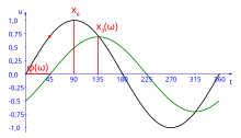
Time course input and output signal

Nyquist diagram of an RC circuit

One can imagine the following experimental setup: A circuit , as an example the series connection of a resistor and a capacitor ( low-pass / RC element ) is driven by a function generator with a sinusoidal voltage applied. The input voltage and the voltage at the capacitor (as output voltage) are measured with an oscilloscope . The following applies at the entrance:

${\displaystyle x_{e}(t)={\hat {x}}_{e}\cdot \sin(\omega \cdot t)}$

The voltage at the output has a different amplitude and a phase shift compared to that at the input:

${\displaystyle x_{a}(t)={\hat {x}}_{a}(\omega )\cdot \sin(\omega \cdot t+\varphi (\omega ))}$

There are:

${\displaystyle \omega }$: Angular frequency of the input voltage,

${\displaystyle x_{e}(t)}$: Instantaneous value of the input voltage,

${\displaystyle x_{a}(t)}$: Instantaneous value of the output voltage,

${\displaystyle {\hat {x}}_{e}}$: Amplitude ( amount ) of the input voltage,

${\displaystyle {\hat {x}}_{a}(\omega )}$: Amplitude (amount) of the output voltage,

${\displaystyle \varphi (\omega )}$: Phase shift ,

${\displaystyle t}$: Time.

If you determine the parameters and for each , the complex frequency response results as: ${\displaystyle \omega }$ ${\displaystyle {\hat {x}}_{a}}$ ${\displaystyle \varphi }$

${\displaystyle F(j\omega )={\frac {x_{a}(j\omega )}{x_{e}(j\omega )}}={\frac {{\hat {x}}_{a}(\omega )}{{\hat {x}}_{e}}}e^{j\varphi (\omega )}}$

The second picture shows the Nyquist diagram of the RC circuit chosen as an example (a PT1 element ). The line labeled with corresponds to a function value dependent on in the complex number level . The locus runs starting from 1 with increasing to the origin and forms a semicircle. The amplitude becomes smaller with increasing , therefore it is a low pass. ${\displaystyle {\frac {x_{a}}{x_{e}}}}$ ${\displaystyle \omega }$ ${\displaystyle \omega }$ ${\displaystyle \omega }$

Compute a Nyquist diagram

A simple PT1 element is used as an example for calculating the Nyqist diagram . To come back to the example with the resistor and the capacitor, is and . ${\displaystyle K_{p}=1}$ ${\displaystyle T_{1}=R\cdot C}$

${\displaystyle F(j\omega )={\frac {K_{p}}{1+j\omega \cdot T_{1}}}}$

The complex number in the denominator can be shortened by complex conjugate expansion:

${\displaystyle F(j\omega )={\frac {K_{p}}{1+j\omega \cdot T_{1}}}\cdot {\frac {1-j\omega \cdot T_{1}}{1-j\omega \cdot T_{1}}}={\frac {K_{p}-j\omega \cdot T_{1}\cdot K_{p}}{1+\omega ^{2}\cdot T_{1}^{2}}}}$

then we get real and imaginary parts:

${\displaystyle \operatorname {Re} \left\{F(j\omega )\right\}={\frac {K_{p}}{1+\omega ^{2}\cdot T_{1}^{2}}}}$,

${\displaystyle \operatorname {Im} \left\{F(j\omega )\right\}={\frac {-\omega \cdot T_{1}\cdot K_{p}}{1+\omega ^{2}\cdot T_{1}^{2}}}}$

This is how the amount and phase are calculated

${\displaystyle |F(j\omega )|={\sqrt {\operatorname {Re} \left\{F(j\omega )\right\}^{2}+\operatorname {Im} \left\{F(j\omega )\right\}^{2}}}={\frac {K_{p}}{\sqrt {1+\omega ^{2}\cdot T_{1}^{2}}}}}$

${\displaystyle \varphi (\omega )=\varphi (F(j\omega ))=\arctan {\frac {\operatorname {Im} \left\{F(j\omega )\right\}}{\operatorname {Re} \left\{F(j\omega )\right\}}}=\arctan(-\omega \cdot T_{1})=-\arctan(\omega \cdot T_{1})}$

The extreme values ​​result as follows:

${\displaystyle \operatorname {Re} \left\{F(j\omega \rightarrow 0)\right\}=K_{p},\quad \operatorname {Im} \left\{F(j\omega \rightarrow 0)\right\}=0}$

${\displaystyle \operatorname {Re} \left\{F(j\omega \rightarrow \infty )\right\}=0,\quad \operatorname {Im} \left\{F(j\omega \rightarrow \infty )\right\}=0}$

${\displaystyle |F(j\omega \rightarrow 0)|=K_{p},\quad \varphi (j\omega \rightarrow 0)=0}$

${\displaystyle |F(j\omega \rightarrow \infty )|=0,\quad \varphi (j\omega \rightarrow \infty )=-90}$

The result is a semicircle like in the graphic above under Experimentally determining a Nyquist diagram .

Draw a Nyquist diagram

To draw a transfer function (Fourier frequency domain):

${\displaystyle H(j\omega )\in \mathbb {C} ,\,\,\omega \in \mathbb {R+} }$

The function is now drawn by simply inserting values ​​for parameters , which results in complex numbers, which are then entered in the diagram and connected. In order to cover a broad spectrum, logarithmically increasing values ​​for and limit value considerations for are useful. In addition, it is useful to calculate the axis interfaces by setting the real or imaginary parts to zero and converting them to. ${\displaystyle \omega }$ ${\displaystyle \omega }$ ${\displaystyle \omega \rightarrow \infty /\omega \rightarrow \ 0}$ ${\displaystyle \omega }$

E.g .: ${\displaystyle \Re \{H(j\omega )\}=0\Rightarrow \omega _{Re0}}$

${\displaystyle \Rightarrow H(j\omega _{Re0})}$ calculate and enter.

Note: The tangent of the Nyquist path in the point is always perpendicular to the real part. ${\displaystyle \omega =0}$

Simplified sketch of the Nyquist locus

In certain cases, a quick sketch of the locus can also be done with a simplified procedure. The transfer function is given in the following form:

${\displaystyle G(s)={\frac {K}{s^{q}}}\cdot {\frac {b_{m}s^{m}+b_{m-1}s^{m-1}+\ldots +b_{1}s+1}{a_{n}s^{n}+a_{n-1}s^{n-1}+\ldots +a_{1}s+1}}e^{-T_{t}s}}$

Additionally, the following conditions must be met: , and the poles and zeros may not be the right of the imaginary axis. The start of the locus for is drawn at an angle of (measured from the real axis), and the locus continues to rotate clockwise until for . When is, the locus rotates monotonically and there is no change in the curvature of the locus. Because of the locus ends at the origin. ${\displaystyle m<q+n}$ ${\displaystyle T_{t}=0}$ ${\displaystyle \omega =0}$ ${\displaystyle -q\cdot 90^{\circ }}$ ${\displaystyle -(q+n-m)\cdot 90^{\circ }}$ ${\displaystyle \omega \rightarrow \infty }$ ${\displaystyle m=0}$ ${\displaystyle m<q+n}$

See also

• Smith Chart
• Phase difference
• Nyquist stability criterion

Web links

• Java applet for the Nyqist diagram