RC element

Under RC elements are understood in the electrical circuits of an ohmic resistance (R -. Engl resistor ) and a capacitor (C - engl. Capacitor ) are constructed. RC elements are linear, time-invariant systems . In a narrower sense, this refers to filters such as the low-pass or high-pass . In the case of a low pass, as in the adjacent picture, the capacitor is connected in parallel at the signal output; in the case of a high pass, capacitor and resistor are swapped.

A capacitor and resistor are connected in parallel for equipotential bonding and functional grounding. To limit electromagnetic interference, there are series connections of capacitor and resistor, such as in the case of the snubber .

Simple RC low pass
U _e : input voltage
U _a : output voltage

Behavior in the time domain

General system-theoretical description of the RC low-pass filter

Voltages and currents at the RC low pass

The RC element in low-pass configuration is an integrating, time-continuous, linear, time-invariant transmission element. The general system-theoretical description results from Kirchhoff's laws, as well as the current / voltage relationships at capacitor or resistor. The mesh equation gives

${\displaystyle -u_{\text{e}}(t)+u_{\text{r}}(t)+u_{\text{c}}(t)=0}$.

Since it is an unbranched circuit, the following applies . The following applies to the voltage drop across the resistor ${\displaystyle i_{\text{c}}(t)=i_{\text{r}}(t)}$

${\displaystyle u_{\text{r}}(t)=Ri_{\text{r}}(t)}$

and the current through the capacitor is through the relationship

${\displaystyle i_{\text{c}}(t)=C{\frac {{\text{d}}u_{\text{c}}(t)}{{\text{d}}t}}}$

set. If we now insert the equation of the voltage across the resistance into the mesh equation, we get

${\displaystyle -u_{\text{e}}(t)+Ri_{\text{r}}(t)+u_{\text{c}}(t)=0}$.

Inserting the current ultimately gives the differential equation

${\displaystyle RC{\frac {{\text{d}}u_{\text{c}}(t)}{{\text{d}}t}}+u_{\text{c}}(t)=u_{\text{e}}(t)}$,

which fully describes the transmission link. In order to clarify the integrating character of the low-pass filter, we will carry out some transformations. The equation is integrated on both sides

${\displaystyle \int RC{\frac {{\text{d}}u_{c}(t)}{{\text{d}}t}}\,{\text{d}}t+\int u_{\text{c}}(t)\,{\text{d}}t=\int u_{\text{e}}(t)\,{\text{d}}t}$,

where the differential and integral operator cancel each other out in a term and follow

${\displaystyle RCu_{\text{c}}(t)+\int u_{\text{c}}(t)\,{\text{d}}t=\int u_{\text{e}}(t)\,{\text{d}}t}$.

Switching according to the output voltage ultimately results ${\displaystyle u_{\text{c}}(t)}$

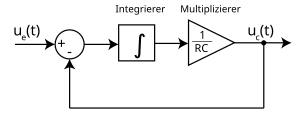
Block diagram of the RC low pass

${\displaystyle u_{\text{c}}(t)={\frac {1}{RC}}\left(\int u_{\text{e}}(t)\,{\text{d}}t-\int u_{\text{c}}(t)\,{\text{d}}t\right)={\frac {1}{RC}}\int \left(u_{\text{e}}(t)\,-u_{\text{c}}(t)\right)\,{\text{d}}t}$.

The integral equation in the time domain can be subjected directly to the Laplace transform , which leads to

${\displaystyle u_{\text{c}}(s)={\frac {1}{RC}}{\frac {1}{\text{s}}}\left(u_{\text{e}}(s)-u_{\text{c}}(s)\right)}$

results. By dividing the output signal by the input signal , the transfer function of the RC low-pass is obtained: ${\displaystyle u_{\text{c}}(t)}$ ${\displaystyle u_{\text{e}}(t)}$

${\displaystyle G_{\text{TP}}(s)={\frac {u_{\text{c}}(s)}{u_{\text{e}}(s)}}={\frac {1}{1+RCs}}}$.

By setting (with the imaginary unit and the angular frequency ) the Fourier transformation and thus the spectral representation of the system results : ${\displaystyle s=\mathrm {j} \omega }$ ${\displaystyle \mathrm {j} }$ ${\displaystyle \omega }$

${\displaystyle G_{\text{TP}}(\mathrm {j} \omega )={\frac {u_{\text{c}}(\mathrm {j} \omega )}{u_{\text{e}}(\mathrm {j} \omega )}}={\frac {1}{1+\mathrm {j} \omega RC}}}$.

The most important class of signals for considering the filter behavior are harmonic signals, so it is often of great interest what attenuation behavior the filter has on a sinusoidal signal. By the input signal

Transient simulation with sinusoidal input signal, R = 1 kΩ, C = 100 nF, f = 5 kHz

${\displaystyle u_{\text{e}}(t)={\hat {u}}\sin(\omega t+\varphi )}$

then follows in the previously derived differential or integral equation

${\displaystyle RC{\frac {{\text{d}}u_{\text{c}}(t)}{{\text{d}}t}}+u_{\text{c}}(t)=u_{\text{e}}(t)={\hat {u}}\sin(\omega t+\varphi )}$.

In order to find the output voltage, you have to switch to, this is analytically possible. It is a linear ordinary differential equation for which there are many different solution methods. If one considers the initial condition , i.e. the case that the system is initially without energy when settling, then the solution is to ${\displaystyle u_{\text{c}}(t)}$ ${\displaystyle u_{\text{c}}(0)=0}$

${\displaystyle u_{\text{c,sin}}(t)={\frac {{\hat {u}}\left(\sin \left(\omega t+\varphi \right)-RC\omega \cos \left(\omega t+\varphi \right)\right)-{\hat {u}}{\text{e}}^{-{\frac {t}{RC}}}\left(\sin(\varphi )-RC\omega \cos(\varphi )\right)}{\left(\omega RC\right)^{2}+1}}}$.

General system-theoretical description of the RC high-pass filter

Voltages and currents at the RC high pass

The RC high-pass is also an unbranched circuit, but the output voltage is tapped at the resistor. In system theory, it is a differentiating transfer element. The mesh equation gives

${\displaystyle -u_{\text{e}}(t)+u_{\text{r}}(t)+u_{\text{c}}(t)=0}$.

The integral relationship applies to the voltage across the capacitor

${\displaystyle u_{\text{c}}(t)={\frac {1}{C}}\int i_{\text{c}}(t)\,{\text{d}}t}$.

Due to the unbranched nature of the circuit , it follows after insertion ${\displaystyle i_{\text{c}}(t)=i_{\text{r}}(t)}$

${\displaystyle -u_{\text{e}}(t)+{\frac {1}{C}}\int i_{\text{r}}(t)\,{\text{d}}t+u_{\text{r}}(t)=0}$.

The current in the integral can be written as :, inserted into the equation follows ${\displaystyle i_{\text{r}}(t)={\frac {u_{\text{r}}(t)}{R}}}$

${\displaystyle -u_{\text{e}}(t)+{\frac {1}{C}}\int {\frac {u_{\text{r}}(t)}{R}}\,{\text{d}}t+u_{\text{r}}(t)=0}$,

this is an integral equation which now fully describes the system. In order to illustrate the differentiating character of the high-pass filter, we will carry out a few more transformations. The equation is differentiated on both sides

${\displaystyle -{\frac {\text{d}}{{\text{d}}t}}u_{\text{e}}(t)+{\frac {1}{C}}{\frac {\text{d}}{{\text{d}}t}}\int {\frac {u_{\text{r}}(t)}{R}}\,{\text{d}}t+{\frac {\text{d}}{{\text{d}}t}}u_{\text{r}}(t)=0}$,

whereby the differential and the integral operator cancel each other out again

${\displaystyle -{\frac {\text{d}}{{\text{d}}t}}u_{\text{e}}(t)+{\frac {1}{RC}}u_{\text{r}}(t)+{\frac {\text{d}}{{\text{d}}t}}u_{\text{r}}(t)=0}$.

Switching to the initial size then results

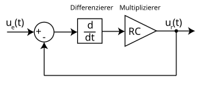
Block diagram of the RC high pass.

${\displaystyle u_{\text{r}}(t)=RC{\frac {\text{d}}{{\text{d}}t}}\left(u_{\text{e}}(t)-u_{\text{r}}(t)\right)}$,

whereby the differentiating behavior becomes evident. The equation can be subjected to the Laplace transform , whereby

${\displaystyle u_{\text{r}}(s)=RCs\left(u_{\text{e}}(s)-u_{\text{r}}(s)\right)}$

follows. The transfer function of the RC high pass is obtained by dividing the output signal by the input signal : ${\displaystyle u_{\text{r}}(t)}$ ${\displaystyle u_{\text{e}}(t)}$

${\displaystyle G_{\text{HP}}(s)={\frac {u_{\text{r}}(s)}{u_{\text{e}}(s)}}={\frac {RCs}{1+RCs}}}$

By setting , the Fourier transformation and thus the spectral representation of the system are obtained: ${\displaystyle s=\mathrm {j} \omega }$

${\displaystyle G_{\text{HP}}(\mathrm {j} \omega )={\frac {u_{\text{r}}(\mathrm {j} \omega )}{u_{\text{e}}(\mathrm {j} \omega )}}={\frac {\mathrm {j} \omega RC}{1+\mathrm {j} \omega RC}}}$.

Here, too, we consider the solution of the differential equation for a harmonic input signal, for which the Laplace transformation can be used. The input signal is

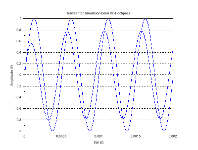
Transient simulation with sinusoidal input signal, R = 1 kΩ, C = 100 nF, f = 2 kHz

${\displaystyle u_{\text{e,sin}}(t)={\hat {u}}\sin(\omega t+\varphi )}$,

whose Laplace transform is

${\displaystyle {\mathcal {L}}\left\{{\hat {u}}\sin(\omega t+\varphi )\right\}={\hat {u}}{\frac {\omega \cos(\varphi )+s\sin(\varphi )}{s^{2}+\omega ^{2}}}}$.

Insertion into the transfer function delivers

${\displaystyle u_{\text{r,sin}}(s)={\frac {RCs}{1+RCs}}{\hat {u}}{\frac {\omega \cos(\varphi )+s\sin(\varphi )}{s^{2}+\omega ^{2}}}}$.

A comprehensive inverse transformation then results in the solution of the differential equation and thus the transient behavior for a sinusoidal input signal:

${\displaystyle u_{\text{r,sin}}(t)={\frac {{\hat {u}}{\text{e}}^{-{\frac {t}{RC}}}\left(\sin(\varphi )-\omega RC\cos(\varphi )\right)+{\hat {u}}\omega RC\left(\cos(\omega t+\varphi )+\omega RC\sin(\omega t+\varphi )\right)}{\left(\omega RC\right)^{2}+1}}}$

Charging process

The system response to a step function is shown here as an example. The voltage is zero volts until the point in time zero and then rises immediately . Current flows into the capacitor until the plates are electrically charged and do not accept any further charge. This occurs when the capacitor voltage U ( t ) equal to the applied voltage U _max is. One plate is then electrically positive, the other negatively charged. There is an excess of electrons on the negatively charged side . ${\displaystyle U_{\rm {max}}}$

The charging time of the capacitor is proportional to the size of the resistor R and the capacitance C of the capacitor. The product of resistance and capacitance is called the time constant . ${\displaystyle \tau }$

${\displaystyle \tau =R\cdot C\,}$

In theory, it takes an infinite amount of time until U (t) = U _max . For practical purposes, the charging time t _L can be used, after which the capacitor can be regarded as approximately fully (more than 99%) charged.

${\displaystyle t_{L}=5\cdot \tau \,}$

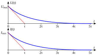
Voltage U and current I curve during the charging process,
U _max is the voltage of the voltage source as the maximum possible voltage

The time constant τ also marks the point in time at which the tangent applied at the beginning of the curve reaches the end value of the voltage. After this time , the capacitor would be charged to its final value if it could be charged with the constant current . In fact, however, the current intensity decreases exponentially over time with a constant applied voltage. ${\displaystyle I_{\rm {max}}}$

The maximum current flows at time t = 0. This results from the resistance R according to Ohm's law , where U _{max is} the applied voltage of the voltage source: ${\displaystyle I_{\rm {max}}}$

${\displaystyle I_{\rm {max}}={\frac {U_{\rm {max}}}{R}}\,}$

The course of the charging voltage U ( t ) or its respective time value is described with the following equation, where e is Euler's number , t is the time after the start of charging and the time constant: ${\displaystyle \tau }$

${\displaystyle U(t)=U_{\rm {max}}\cdot (1-e^{-{\frac {t}{\tau }}})\,}$,

It is assumed that the capacitor at the beginning was not charged: . The voltage is therefore zero at first and then increases in the form of an exponential function . After this time , the voltage has reached about 63% of the applied voltage U _max . After the time the capacitor is charged to more than 99%. ${\displaystyle U(t=0)=0}$ ${\displaystyle t=\tau }$ ${\displaystyle t=5\tau }$

The course of the current intensity I ( t ) or its respective time value is described with the following equation:

${\displaystyle I(t)=I_{\rm {max}}\cdot e^{-{\frac {t}{\tau }}}\,}$

Here the current is at the first moment and then decreases in the form of an exponential function like during the discharge process. After the time the current is only about 37% of its initial value and after the time it has dropped to less than 1%. ${\displaystyle I(t=0)=I_{\rm {max}}}$ ${\displaystyle t=\tau }$ ${\displaystyle t=5\tau }$

Differential equation of the charging process

The following applies to the charging process of the capacitor for an ideal voltage source with the voltage : ${\displaystyle E}$

${\displaystyle Q(t)=EC\cdot \left(1-e^{-{\frac {t}{RC}}}\right)}$

This is derived as follows. The following applies to the current:

${\displaystyle I(t)={\frac {\mathrm {d} Q(t)}{\mathrm {d} t}}={\dot {Q}}(t)}$

The following applies to the voltage at the ohmic resistor:

${\displaystyle U_{R}=R\cdot I(t)=R\cdot {\dot {Q}}(t)}$

The following applies to the voltage across the capacitor:

${\displaystyle U_{C}={\frac {Q(t)}{C}}}$

For a simple circuit consisting of a capacitor and an ohmic resistor, the following applies according to the mesh set :

${\displaystyle {\begin{array}{crcl}&U_{C}+U_{R}&=&E\\\Leftrightarrow &{\frac {Q(t)}{C}}+R\cdot {\dot {Q}}(t)&=&E\\\Leftrightarrow &{\frac {1}{RC}}\cdot Q(t)+{\dot {Q}}(t)&=&{\frac {E}{R}}\\\end{array}}}$

This differential equation is solved by first solving the homogeneous equation by first setting: ${\displaystyle E/R=0}$

${\displaystyle \int _{t_{0}}^{t}{\frac {{\dot {Q}}(t)}{Q(t)}}\,\mathrm {d} t=\int _{t_{0}}^{t}-{\frac {1}{RC}}\,\mathrm {d} t}$

Since is constant, the following applies: ${\displaystyle -{\tfrac {1}{RC}}}$

${\displaystyle \int _{t_{0}}^{t}{\frac {{\dot {Q}}(t)}{Q(t)}}\,\mathrm {d} t=-{\frac {1}{RC}}\int _{t_{0}}^{t}1\,\mathrm {d} t}$

According to the substitution rule:

${\displaystyle \ln \left|Q(t)\right|-\ln \left|Q(t_{0})\right|=-{\frac {t-t_{0}}{RC}}}$

${\displaystyle Q_{v}}$is the anticipated name for the method used in the next steps variation of the constants , is the electrical charge of the capacitor at the point in time , it cannot become negative, is the point in time at the beginning of charging and has the value 0 s; it follows: ${\displaystyle Q(t)}$ ${\displaystyle t}$ ${\displaystyle t_{0}}$

${\displaystyle \ln \left({\frac {Q(t)}{Q_{v}}}\right)=-{\frac {t}{RC}}}$

By raising the base e to the power of:

${\displaystyle {\frac {Q(t)}{Q_{v}}}=e^{-{\frac {t}{RC}}}\Leftrightarrow Q(t)=Q_{v}\cdot e^{-{\frac {t}{RC}}}}$

In order to be able to solve the inhomogeneous differential equation now, we apply the method of varying the constants by considering them as time-dependent and inserting them as they are and differentiated into the output equation. ${\displaystyle Q_{v}(t)}$

${\displaystyle {\dot {Q}}(t)={\dot {Q}}_{v}(t)\cdot e^{-{\frac {t}{RC}}}-{\frac {Q_{v}(t)}{RC}}\cdot e^{-{\frac {t}{RC}}}}$

use in:

${\displaystyle {\begin{array}{rcl}{\frac {E}{R}}&=&{\frac {1}{RC}}\cdot Q(t)+{\dot {Q}}(t)\\&=&{\frac {Q_{v}(t)}{RC}}\cdot e^{-{\frac {t}{RC}}}+{\dot {Q}}_{v}(t)\cdot e^{-{\frac {t}{RC}}}-{\frac {Q_{v}(t)}{RC}}\cdot e^{-{\frac {t}{RC}}}\\&=&{\dot {Q}}_{v}(t)\cdot e^{-{\frac {t}{RC}}}\\\end{array}}}$

This will be converted and integrated according to: ${\displaystyle {\dot {Q}}_{v}(t)}$

${\displaystyle {\begin{array}{rcl}\int _{t_{0}}^{t}{\dot {Q}}_{v}(t)\,\mathrm {d} t&=&\int _{t_{0}}^{t}{\frac {E}{R}}\cdot e^{\frac {t}{RC}}\,\mathrm {d} t\\Q_{v}(t)-Q_{v}(t_{0})&=&{\frac {E}{R}}\cdot RC\left(e^{\frac {t}{RC}}-e^{\frac {t_{0}}{RC}}\right)\end{array}}}$

As mentioned above, charging starts at the point in time . At this point the charge on the capacitor is : ${\displaystyle t_{0}=0}$ ${\displaystyle Q_{v}(t_{0})=0}$

${\displaystyle {\begin{array}{rcl}Q_{v}(t)-0&=&EC\left(e^{\frac {t}{RC}}-e^{\frac {0}{RC}}\right)\\Q_{v}(t)&=&EC\cdot \left(e^{\frac {t}{RC}}-1\right)\\\end{array}}}$

That has to be put into the solution of the DGL:

${\displaystyle {\begin{array}{rcl}Q(t)&=&Q_{v}\cdot e^{-{\frac {t}{RC}}}\\&=&EC\cdot \left(e^{\frac {t}{RC}}-1\right)\cdot e^{-{\frac {t}{RC}}}\\&=&EC\cdot \left(1-e^{-{\frac {t}{RC}}}\right)\end{array}}}$

That is the equation as it is above. If you choose a theoretically fully charged capacitor as the value, the equation becomes: ${\displaystyle EC=Q_{E}}$

${\displaystyle Q(t)=Q_{E}\cdot \left(1-e^{-{\frac {t}{RC}}}\right)}$

The same applies to the voltage : ${\displaystyle U}$

${\displaystyle U(t)={\frac {Q(t)}{C}}=E\cdot \left(1-e^{-{\frac {t}{RC}}}\right)}$

and for the amperage : ${\displaystyle I(t)}$

${\displaystyle I(t)={\dot {Q}}(t)=\left({\frac {EC}{RC}}\right)\cdot e^{-{\frac {t}{RC}}}=I_{0}\cdot e^{-{\frac {t}{RC}}}}$

Unloading process

Course of voltage U and current I during the discharge process,
U _max is the initial voltage

The picture shows the discharge process when the capacitor is initially charged to the value U _max and is discharged through the resistor R. Both the voltage and the current are greatest here at the beginning:

For t = 0 the following applies:    and is at any point in time thereafter    ${\displaystyle I_{\rm {max}}={\frac {U_{\rm {max}}}{R}}}$ ${\displaystyle I(t)={\frac {U(t)}{R}}}$

The voltage decreases over time according to the course of the discharge

${\displaystyle U(t)=U_{\rm {max}}\cdot e^{-{\frac {t}{\tau }}}\,}$

The current that is linked to the voltage U (t) via the discharge resistor R shows the corresponding curve

${\displaystyle I(t)=I_{\rm {max}}\cdot e^{-{\frac {t}{\tau }}}\,}$

The discharge current is negative in the specified direction of the counting arrow.

Differential equation of discharge

The following applies to the discharge process of the capacitor:

${\displaystyle Q(t)=Q_{0}\cdot e^{-{\frac {t}{RC}}}}$

This is derived like the charging process. The solved differential equation can be taken from there. The initial conditions are just different and the method of varying the constants is not required:

${\displaystyle \ln \left|Q(t)\right|-\ln \left|Q(t_{0})\right|=-{\frac {t-t_{0}}{RC}}}$

${\displaystyle Q(t)}$is the electrical charge of the capacitor at the point in time , it cannot become negative, is the point in time at the beginning of the discharge and has the value 0 s. There is no discharge here, but an initial charge ; it follows: ${\displaystyle t}$ ${\displaystyle t_{0}}$ ${\displaystyle Q_{0}}$

${\displaystyle \ln \left({\frac {Q(t)}{Q(0)}}\right)=-{\frac {t}{RC}}}$

By raising the base e to the power of:

${\displaystyle {\frac {Q(t)}{Q_{0}}}=e^{-{\frac {t}{RC}}}\Leftrightarrow Q(t)=Q_{0}\cdot e^{-{\frac {t}{RC}}}}$

The same applies to the voltage : ${\displaystyle U}$

${\displaystyle U(t)={\frac {Q(t)}{C}}=U_{0}\cdot e^{-{\frac {t}{RC}}}}$

and for the amperage : ${\displaystyle I}$

${\displaystyle I(t)={\dot {Q}}(t)=-I_{0}\cdot e^{-{\frac {t}{RC}}}}$

Impulse response

Course of charging current (blue) and capacitor voltage (pink) on an RC element on a voltage pulse

The impulse response describes the output voltage curve on a direct pulse-shaped input voltage. The output voltage curve is described by its time derivative:

${\displaystyle {\dot {U}}(t)={\frac {dU}{dt}}={\frac {U_{q}}{\tau }}e^{-{\frac {t}{\tau }}}\,}$

This is the instantaneous voltage across the resistor that causes the capacitor to charge. The voltage pulse is integrated by the RC element and leaves a capacitor charge, which is then discharged in the form of an exponential function. ${\displaystyle {U_{q}}}$

The rate of voltage rise (volts per second) is an important variable in electronics and power electronics. ${\displaystyle {\frac {dU}{dt}}}$

Periodic signals

Time curve of the voltage (blue) across a capacitor, which is periodically charged and discharged via a resistor from an ideal square-wave voltage source (red)

The filter effect becomes particularly clear with square-wave signals; the filter response is made up of segments of the charging and discharging behavior. The edge steepness is lower, and accordingly high frequencies are missing in the frequency spectrum. RC elements are used accordingly for interference suppression and as a low pass .

The edge steepness of the voltage on the capacitor with an amplitude U _{0 of} the square-wave voltage source drops from the infinite value of the feeding square-wave voltage to a maximum

${\displaystyle {\frac {dU}{dt}}={\frac {U_{0}}{RC}}={\frac {U_{0}}{\tau }}}$.

from. The maximum charging current (peak current, pulse current I _p ) is

${\displaystyle {I_{p}}={\frac {U_{0}}{R}}}$.

Switching contacts or semiconductor switches connected to an RC suppressor , for example, must be able to withstand this current .

Behavior in the frequency domain

Low pass

Amplitude response of an RC low-pass filter. The ordinate shows the amplitude ratio in decibels , the abscissa the normalized angular frequency Ω in a logarithmic representation . ${\displaystyle |H|}$

Phase shift as a function of the normalized frequency Ω at the RC element.

Phase shift of 90 ° between current and voltage on the capacitor

Z, R, Xc

V, Vr, Vc

Resistor and capacitor form a frequency-dependent voltage divider , which also causes a phase shift of a maximum (90 °). The impedances Z are R and . For the RC element, the following applies to a harmonic oscillating voltage of the frequency : ${\displaystyle {\frac {\pi }{2}}}$ ${\displaystyle 1/(\mathrm {j} \omega C)}$ ${\displaystyle f={\frac {\omega }{2\pi }}}$

${\displaystyle U_{a}=U_{e}\cdot {\frac {Z_{C}}{Z_{R}+Z_{C}}}\,}$

and thus for the transmission behavior , which is defined as the quotient of output to input voltage:

${\displaystyle H={\frac {U_{a}}{U_{e}}}={\frac {Z_{C}}{Z_{R}+Z_{C}}}={\frac {\frac {1}{\mathrm {j} \omega C}}{R+{\frac {1}{\mathrm {j} \omega C}}}}={\frac {1}{1+\mathrm {j} \omega RC}}={\frac {1}{1+\mathrm {j} {\mathit {\Omega }}}}\,}$,

where the normalized frequency Ω = ω / ω ₀ results from the division of the angular frequency ω = 2π f and the limit angular frequency (transition frequency, cutoff frequency ) ω _c = 1 / τ = 1 / ( RC ). This results in the cut-off frequency f _c , at which reactance and resistance assume the same value, i.e. the phase shift (45 °) and the attenuation is around 3 dB: ${\displaystyle {\frac {\pi }{4}}}$

${\displaystyle f_{c}={\frac {1}{2\pi \cdot R\cdot C}}\,}$

For low frequencies Ω  << 1, H is about 1, input and output voltage about the same, which is why the range is also called called the pass band .
For frequencies Ω  >> 1, H drops by 20 dB per decade = 6 dB per octave. The area filtered out is called the stop band .

At very low frequencies, which are significantly lower than the cut-off frequency, the charging current of the capacitor is irrelevant and the input and output voltage differ only imperceptibly. The phase shift is approximately 0 °.

If the frequency increases, it takes longer - compared to the period of oscillation - until the capacitor is charged to the input voltage. Therefore the phase shift increases.

At a very high frequency, this tends towards the limit value of 90 °, but then the voltage on the capacitor is also immeasurably small.

High pass

The interconnection of a high-pass differs from that of the low-pass filter by interchanging R and C . Accordingly,

${\displaystyle U_{a}=U_{e}\cdot {\frac {Z_{R}}{Z_{C}+Z_{R}}}\,}$

and

${\displaystyle H={\frac {U_{a}}{U_{e}}}={\frac {Z_{R}}{Z_{C}+Z_{R}}}={\frac {R}{{\frac {1}{\mathrm {j} \omega C}}+R}}={\frac {\mathrm {j} \omega RC}{1+\mathrm {j} \omega RC}}={\frac {\mathrm {j} {\mathit {\Omega }}}{1+\mathrm {j} {\mathit {\Omega }}}}\,}$,

The amplitude response is  mirrored in relation to the low pass along Ω = 1, high frequencies can pass almost undamped.

Description in the spectral range

With an analog derivation one obtains for the low pass

${\displaystyle H(s)={\frac {1}{1+sRC}}\,}$,

a pole at . ${\displaystyle s=-1/RC}$

At the high pass

${\displaystyle H(s)={\frac {sRC}{1+sRC}}\,}$,

there is also a pole at , plus a zero at the origin. The RC element thus represents a 1st order Butterworth filter . ${\displaystyle s=-1/RC}$

Web links

• RC element calculation of transition frequency and time constant
• Animation of the charging and discharging of the capacitor