Geometric modeling
Geometric modeling, also English computer-aided geometric design known (CAGD), refers to the computer-based description of the shape of geometric objects. It deals with the description of two-dimensional curves as well as three-dimensional surfaces and bodies . Geometric modeling is used in computer graphics , computer-aided design (CAD), the finite element method and other engineering and scientific areas.

Freeform curves and surfaces
Free-form curves and surfaces can be described by means of splines , meaning here piecewise polynomial functions. The principle can be extended from the two-dimensional curves to three-dimensional surfaces.
Hermite curves
Cubic Hermitian curves are composed of third degree Hermitian polynomials . Each polynomial is determined by a start and end point and the corresponding tangent. When the Hermitian polynomials are put together to form a spline, the tangents of two adjacent polygons are set equal. There are various options for choosing the tangents. The simplest is to equate a tangent with the straight line connecting the nearest control points, but other methods have been developed:
- With cardinal splines , the tangents are determined by a parameter c between 0 and 1, which specifies the "tension" at the control point.
- Catmull-Rom splines are a special case of cardinal splines, where c = 0. They are oftenused as animationcurves in computer animation because they run precisely through the control points and their derivation is continuous .
- Kochanek-Bartels splines , also called TCB splines, offer a further parameterization of Hermite curves with the three parameters of tension, continuity and bias.
Bezier curves
An n- th degree Bézier curve is a parametric curve defined by n +1 control points. The polygon that connects the control points is called the control polygon. While a linear Bézier curve, i.e. a Bézier curve of the first degree, is a simple segment between the two control points, a quadratic Bézier curve describes a part of a parabola . Many graphics programs use cubic Bezier curves.
A Bézier curve interpolates between the individual control points using Bernstein polynomials , which indicate the influence of the control points as a function of the curve parameters. Apart from the start and end points, the curve generally does not pass through the control points, but is contained in their convex hull . The De Casteljau algorithm can be used to draw a Bézier curve, which approximates a Bézier curve by means of a polygon.
Bézier curves are invariant under affine maps . This means that an affine mapping of the control points produces the same curve as an affine mapping of the original curve. A problem with Bézier curves is that, given a certain position of the control points, touch points or colons are possible. Local changes to the control points have an undesirable effect on the entire curve, but are only of local importance.
B-spline curves and NURBS
Compared to Bézier curves, B-spline curves offer better locality and controllability: Changes only have a local effect and only part of the curve has to be recalculated. Similar to Hermite curves, B-spline curves are pieced together from individual polynomials. The seams are called nodes . Undesired oscillations ( Runge's phenomenon ) with a large number of nodes are thus avoided. B-spline curves are a linearly weighted combination of basic functions called B-splines. The basis functions are piecewise polynomials with a small carrier . Changes outside the beam do not affect the B-spline curve.
Uniform basic functions are shifted copies of one another, each centered on a node. Uniform, linear basis functions are triangular functions that are centered at a certain node and have a support that extends over three nodes. Quadratic and cubic basis functions are composed of correspondingly higher polynomials, but always centered over a node. In contrast, non-uniform basis functions have different forms. B-spline curves can be converted into a polygon using the De-Boor algorithm .
An extension are rational B-spline curves or in general Non-Uniform Rational B-Splines (NURBS), the parametric representation of which is a mathematical fraction. NURBS are general enough to describe all common curves and surfaces. Some newer modeling tools use it as the sole internal method of representation.
Representation schemes
Various methods for representing bodies (representation schemes) have been developed which differ in terms of their storage requirements, numerical precision, complexity and the ability to be converted into other representation schemes. Another property of a representation scheme is the ability to check whether a model is correct, ie a “real”, physically possible object is defined.
A distinction is made between direct representation schemes, which describe the volume itself, and indirect schemes, in which the description takes place via edges and surfaces. Hybrid schemes that combine both methods are also conceivable.
Direct representation schemes
Norm cell enumeration scheme
In the norm cell enumeration scheme, the space is divided into an evenly divided grid of cells ( voxels ). A body is represented by a set of cells. The smaller the voxels, the better the body approximates. The enumeration scheme takes up a lot of memory.
Constructive Solid Geometry
With Constructive Solid Geometry (CSG), objects are modeled with the help of basic bodies such as spheres, cuboids or cylinders as well as operators such as intersection, union or difference. A CSG body can be described using a formula that applies the operators to basic bodies and illustrated as a tree.
CSG is particularly common in the CAD area. An investigation came to the result that 63% of all mechanical components can be modeled with a CSG system that only uses cuboids and straight circular cylinders . If more base bodies are permitted, 90% of all components in classic mechanical engineering (primarily drilling , milling , turning of the components or their molds) can be described naturally using CSG.
A great advantage of CSG compared to other display schemes is that their correctness is guaranteed, provided that only certain basic bodies are permitted. If, for example, R-sets are used as the basic body, their properties guarantee that a corresponding CSG tree is correct. In addition, CSG bodies are very compact and easy to produce. However, many rendering methods cannot deal with CSG directly and require CSG bodies to be converted to B-reps first, which is a comparatively difficult task.
Until the 1980s, most modeling tools were based either on Boundary Representations or on CSG.
Generative modeling
A generative model is a shape created by continuously transforming a shape called a generator . The dimension of the model does not matter. The modeling takes place at a high level and is expandable. With the help of a programming language like Generative Modeling Language , the user can easily build a library of useful shapes.
Shift geometries, also called sweeps , are a special case of generative models. They are created by moving a curve or volume along a curve.
A special case of sweeps are surfaces of revolution that are created by rotating a certain amount around any axis.
Voxel grid
Voxel grids are spatial and grid-like arranged values that describe the "density" of an object and can be represented using the means of volume graphics . Voxel grids make it possible to "cut away" parts of objects and see inside. CSG operations are also easy to implement. However, voxel gratings require a great deal of storage space and they tend to have undesirable aliasing effects. In some applications, the increased memory requirement can be reduced by using octrees . Modeling using voxel grids is mainly used in medicine, fluid dynamics and the representation of natural objects such as clouds.
Indirect representation schemes
Wireframe model

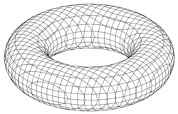
A wireframe model defines a body solely by its edges. This model offers advantages in terms of speed, as the display is very efficient. One problem with this scheme is its ambiguity. A wireframe model can represent several different bodies because it is not clear where the surfaces are. A concealment calculation as with surfaces is therefore not possible, but the haloed line algorithm can be used.
Surface rendering
A surface representation, also called Boundary Representation or B-rep , is the description of a body based on its surface; B-reps are therefore "hollow". B-reps are probably the most common representation scheme used in computer graphics. Polygon networks in particular are often used.
B-reps are well suited for efficient rendering of general surfaces and allow local changes to be made to the model. Disadvantages of B-reps are their high memory requirements and the difficulty in verifying their correctness.
Representation schemes based on so-called Euler operations are used to at least partially guarantee correctness when modeling bodies as B-rep. The idea is to only allow so-called Euler operations that retain the Euler characteristics or change them in a certain way.
Modeling techniques
Polygonization
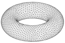
Many algorithms in computer graphics, including some rendering methods, work exclusively with polygon meshes. Also finite element methods based on this presentation. Numerous polygonization algorithms have been developed that produce results of varying quality. In general, a polygonization method should achieve a good approximation of the shape of the original object, produce polygons with a balanced shape that is not too narrow, and respect the local topology of the original object, i.e. not create any gaps or breaks. Examples of polygonization algorithms are
- the cutting cube algorithm by M. Schmidt and
- the tracking algorithm of E. Hartmann. Please refer
Physically based modeling
Modeling methods that take into account the dynamic properties of objects in addition to the static ones are called physically based. Objects can not only be rigid, but also flexible. An example is a piece of fabric that is placed over other objects and the folds of which are calculated automatically.
See also
literature
- Stephan Abramowski, Heinrich Müller: Geometric modeling. BI Wissenschaftsverlag, Mannheim 1991
- Max Agoston: Computer Graphics and Geometric Modeling: Implementation and Algorithms. Springer, London 2005, ISBN 1-85233-818-0
- Max Agoston: Computer Graphics and Geometric Modeling: Mathematics. Springer, London 2005, ISBN 1-85233-817-2
- Gerald Farin: Curves and Surfaces for Computer-Aided Geometric Design. Academic Press, San Diego 1997, ISBN 0-12-249054-1
- Josef Hoschek, Dieter Lasser: Basics of geometric data processing. Teubner, Stuttgart 1992, ISBN 3-519-12962-0
- Michael Mortenson: Geometric Modeling. Industrial Press, New York 2006, ISBN 0-8311-3298-1
Web links
- Erich Hartmann: Geometry and Algorithms for CAD . (PDF; 2.87 MB) Lecture Note, 2003, TU Darmstadt
- Basics of free-form geometry for climate and terrain modeling . (PDF; ~ 700 kB) Summary, 2015, Vienna
References and comments
- ↑ “B-splines” are often used to describe not only the basic functions, but also the B-spline curves that are composed of them. The terms “basic functions” and “B-spline curves” are used here to differentiate.
- ↑ MM Samuel et al. a .: Methodology and Results of an Industrial Parts Survey. In: Technical Memorandum 21, Production Automation Project, University of Rochester, New York 1976. Quoted in Max Agoston: Computer Graphics and Geometric Modeling: Implementation and Algorithms, p. 169
- ^ Max Agoston: Computer Graphics and Geometric Modeling: Implementation and Algorithms, p. 166
- ^ M. Schmidt: Cutting Cubes - visualizing implicit surfaces by adaptive polygonization . Visual Computer (1993) 10, pp. 101-115
- ^ E. Hartmann: A marching method for the triangulation of surfaces , The Visual Computer (1998), 14, pp. 95-108
- ↑ Geometry and Algorithms for COMPUTER AIDED DESIGN , p. 81


