Gaussian process

A Gaussian process (after Carl Friedrich Gauß ) is a stochastic process in probability theory , in which every finite subset of random variables is multidimensionally normally distributed (Gaussian distributed). Generally speaking, a Gaussian process represents temporal, spatial or any other functions whose function values ​​can only be modeled with certain uncertainties and probabilities due to incomplete information. It is constructed from functions of the expected values , variances and covariances and thus describes the function values ​​as a continuum of correlated random variables in the form of an infinite-dimensional normal distribution. A Gaussian process is thus a probability distribution of functions. A random sample results in a random function with certain preferred properties.

Applications

Gaussian processes are used for the mathematical modeling of the behavior of non-deterministic systems on the basis of observations. Gaussian processes are suitable for signal analysis and synthesis, form a powerful tool for interpolation , extrapolation or smoothing of any dimensional discrete measurement points (Gaussian process regression or kriging method) and are used in classification problems . Like a monitored machine learning process, Gaussian processes can be used for abstract modeling on the basis of training examples, with no iterative training being necessary as with neural networks . Instead, Gaussian processes are derived very efficiently using linear algebra from statistical values ​​in the examples and are mathematically clearly interpretable and easy to control. In addition, an associated confidence interval is calculated for each individual output value, which precisely estimates its own prediction error, while known errors in the input values ​​are correctly propagated.

Mathematical description

definition

A Gaussian process is a special stochastic process on an arbitrary index set if its finite-dimensional distributions are multi-dimensional normal distributions (also Gaussian distributions). So the multivariate distribution of through a -dimensional normal distribution should be given for all . ${\displaystyle (X_{t})_{t\in T}}$ ${\displaystyle T}$ ${\displaystyle t_{1},t_{2},\dotsc ,t_{n}\in T}$ ${\displaystyle (X_{t_{1}},X_{t_{2}},\dotsc ,X_{t_{n}})}$ ${\displaystyle n}$

Term: Although the word process is associated with a temporal process for historical reasons , a stochastic process or Gaussian process is only the mathematical description of an indeterminacy of any continuous functions. A Gaussian process is to be understood as a probability distribution. A more appropriate name would be, for example, Gaussian continuum .

notation

Analogous to the one- and multi-dimensional Gaussian distribution, a Gaussian process is completely and uniquely determined via its first two moments . In the multi-dimensional Gaussian distribution, these are the expectation value vector and the covariance matrix . In the Gaussian process, they are replaced by an expected value function and a covariance function . In the simplest case, these functions can be understood as a vector with continuous rows or as a matrix with continuous rows and columns. The following table compares one-dimensional and multi-dimensional Gaussian distributions with Gaussian processes. The symbol can be read as " is distributed like ". ${\displaystyle {\vec {\mu }}}$ ${\displaystyle \Sigma }$ ${\displaystyle m(t):=\mathbb {E} (X_{t})}$ ${\displaystyle k(t,t'):=\operatorname {Cov} (X_{t},X_{t'})}$ ${\displaystyle :=\mathbb {E} \left[(X_{t}-\mathbb {E} (X_{t}))\cdot (X_{t'}-\mathbb {E} (X_{t'}))\right]}$ ${\displaystyle \sim }$

Type of distribution	notation	Sizes	Probability density function
One-dimensional Gaussian distribution	${\displaystyle X\sim {\mathcal {N}}(\mu ,\sigma ^{2})}$	${\displaystyle X,\mu ,\sigma \in \mathbb {R} }$	${\displaystyle p(x)={\frac {1}{\sigma {\sqrt {2\pi }}}}\exp {\bigl \lbrace }-{\tfrac {1}{2}}(x-\mu )^{2}/{\sigma ^{2}}{\bigr \rbrace }}$
Multi-dimensional Gaussian distribution	${\displaystyle {\vec {X}}\sim {\mathcal {N}}_{n}({\vec {\mu }},\Sigma )}$	${\displaystyle {\vec {X}},{\vec {\mu }}\in \mathbb {R} ^{n};\Sigma \in \mathbb {R} ^{n\times n}}$	${\displaystyle p({\vec {x}})={\frac {1}{(2\pi )^{\frac {n}{2}}|\Sigma |^{\frac {1}{2}}}}\exp {\bigl \lbrace }-{\tfrac {1}{2}}({\vec {x}}-{\vec {\mu }})^{T}\Sigma ^{-1}({\vec {x}}-{\vec {\mu }}){\bigr \rbrace }}$
Gaussian process	${\displaystyle (X_{t})\sim {\mathcal {GP}}(m,k)}$	${\displaystyle m\colon T\to \mathbb {R} }$ ${\displaystyle k\colon T\times T\to \mathbb {R} }$	(no analytical representation)

The probability density function of a Gaussian process cannot be represented analytically because there is no corresponding notation for operations with continuous matrices. This gives the impression that one cannot calculate with Gaussian processes like with finite-dimensional normal distributions. In fact, the essential property of the Gaussian process is not the infinity of dimensions, but rather the assignment of the dimensions to certain coordinates of a function. In practical applications you only have to deal with a finite number of support points and you can therefore carry out all calculations as in the finite-dimensional case. The limit value for an infinite number of dimensions is only required in an intermediate step, namely when values ​​are to be read out at new interpolated support points. In this intermediate step, the Gaussian process, i.e. H. the expected value function and covariance function, represented or approximated by suitable analytical expressions. The assignment to the interpolation points takes place directly via the parameterized coordinates in the analytical printout. In the finite-dimensional case with discrete support points, the noted coordinates are assigned to the dimensions via their indices. ${\displaystyle t}$ ${\displaystyle t_{i}}$

Example of a Gaussian process

As a simple example, consider a Gaussian process

${\displaystyle (X_{t})\sim {\mathcal {GP}}(m,k)}$

with a scalar variable (time) through the expected value function ${\displaystyle t}$

${\displaystyle m(t)=5\,{\text{Volt}}}$

and covariance function

${\displaystyle k(t,t')={\begin{cases}(1\,{\text{Volt}})^{2}&t=t'\\0&t\neq t'\end{cases}}}$

given. This Gaussian process describes an endless time electrical signal with Gaussian white noise with a standard deviation of one volt around a mean voltage of 5 volts.

Definitions of special properties

A Gaussian process is called centered if its expectation value is constant 0, i.e. if for all . ${\displaystyle m(t):=\mathbb {E} (X_{t})=0}$ ${\displaystyle t\in T}$

A Gaussian process is called stationary if its covariance function is translation invariant, i.e. it can be described by a relative function . ${\displaystyle k(t,t'):=\operatorname {Cov} (X_{t},X_{t'})}$ ${\displaystyle k(t,t')=k(t-t')}$

A Gaussian process with isotropic properties is called radial if its covariance function can be described by a radially symmetric and also stationary function with a one-dimensional parameter using the Euclidean norm . ${\displaystyle k(t,t')=k(\|t-t'\|)}$ ${\displaystyle \|\cdot \|}$

List of common Gaussian processes and covariance functions

• Constant: and ${\displaystyle m(t)=0}$ ${\displaystyle k(t,t')=\sigma ^{2}}$

Corresponds to a constant value from a Gaussian distribution with standard deviation . ${\displaystyle \sigma }$

• Offset: and ${\displaystyle m(t)=c}$ ${\displaystyle k(t,t')=0}$

Corresponds to a constant value that is fixed by . ${\displaystyle c}$

• Gaussian white noise : ${\displaystyle k(t,t')=\sigma ^{2}\delta _{t,t'}}$

( Standard deviation : Kronecker delta ) ${\displaystyle \sigma }$ ${\displaystyle \delta }$

• Rationally square: ${\displaystyle k(r)=(1+r^{2})^{-\alpha },\quad \alpha \geq 0}$
• Gamma exponential: ${\displaystyle k(r)=\exp \left(-\left({\frac {r}{\ell }}\right)^{\gamma }\right)}$
• Ornstein-Uhlenbeck / Gauß-Markov : ${\displaystyle k(r)=\exp \left(-{\frac {r}{\ell }}\right)}$

Describes continuous, non-differentiable functions, as well as white noise after it has passed through an RC low-pass filter.

• Quadratic exponential: ${\displaystyle k(r)=\exp {\Big (}-{\frac {r^{2}}{2\ell ^{2}}}{\Big )}}$

Describes smooth functions that are infinitely differentiable.

• Matérn:

${\displaystyle k_{\nu =p+1/2}(r)=\exp \left(-{\frac {{\sqrt {2\nu }}r}{\ell }}\right){\frac {\Gamma (p+1)}{\Gamma (2p+1)}}\sum _{i=0}^{p}{\frac {(p+i)!}{i!(p-i)!}}\left({\frac {{\sqrt {8\nu }}r}{\ell }}\right)^{p-i}}$

Very universally applicable Gaussian processes for describing most of the typical measurement curves. The functions of the Gaussian process are -time continuously differentiable, if . Common special cases are: ${\displaystyle n}$ ${\displaystyle \nu >n}$

${\displaystyle k_{\nu =3/2}(r)=\left(1+{\frac {{\sqrt {3}}r}{\ell }}\right)\exp \left(-{\frac {{\sqrt {3}}r}{\ell }}\right)}$

${\displaystyle k_{\nu =5/2}(r)=\left(1+{\frac {{\sqrt {5}}r}{\ell }}+{\frac {{\sqrt {5}}r^{2}}{3\ell ^{2}}}\right)\exp \left(-{\frac {{\sqrt {5}}r}{\ell }}\right)}$

${\displaystyle k_{\nu =1/2}(r)}$corresponds to the Ornstein-Uhlenbeck covariance function and the quadratic exponential. ${\displaystyle k_{\nu \rightarrow \infty }(r)}$

• Periodically: ${\displaystyle k(r)=\exp \left(-{\frac {2\sin ^{2}\left(\pi {\frac {r}{T}}\right)}{\ell ^{2}}}\right)}$

Functions from this Gaussian process are both periodic with the period duration and smooth (quadratic exponential). ${\displaystyle T}$

• Polynomial: ${\displaystyle k(t,t')=\left(t^{\top }t'+\sigma _{0}^{2}\right)^{p}}$

Outwardly grows a lot and is usually a poor choice for regression problems, but can be useful for high-dimensional classification problems. It is positive semidefinite and does not necessarily generate invertible covariance matrices.

• Brownian bridge : and ${\displaystyle m(t)=0}$ ${\displaystyle k(t,t')=\min(t,t')-tt'}$
• Wiener process : and ${\displaystyle m(t)=0}$ ${\displaystyle k(t,t')=\min(t,t')}$

Corresponds to the Brownian movement

• Ito process : Ifand,two integrable real-valued functions anda Wiener process, then the Ito process ${\displaystyle T=\mathbb {R} _{+}}$ ${\displaystyle f}$ ${\displaystyle g}$ ${\displaystyle (W_{t})}$

${\displaystyle X_{t}=\int _{0}^{t}f(s)\,\mathrm {d} s+\int _{0}^{t}g(s)\,\mathrm {d} W_{s}}$

a Gaussian process with and . ${\displaystyle m(t)=\int _{0}^{t}f(s)\,\mathrm {d} s}$ ${\displaystyle k(t,t')=\int _{0}^{\min(t,{t'})}g^{2}(s)\,\mathrm {d} s}$

Remarks:

• ${\displaystyle r:=\|t-t'\|}$ is the distance for stationary and radial covariance functions ${\displaystyle k(t,t')=k(r)}$
• ${\displaystyle \ell }$is the characteristic length scale of the covariance function for which the correlation has dropped to about . ${\displaystyle e^{-1}}$
• Most stationary covariance functions are noted as normalized and are therefore equivalent to correlation functions . For use as a covariance function, they are multiplied by a variance , which assigns a scaling and / or physical unit to the variables. ${\displaystyle k(r)}$ ${\displaystyle k(0)=1}$ ${\displaystyle \sigma ^{2}}$
• Covariance functions must not be arbitrary functions or , since it must be ensured that they are positive definite . Positive semidefinite functions are also valid covariance functions, whereby it should be noted that these do not necessarily result in invertible covariance matrices and are therefore usually combined with a positively definite function. ${\displaystyle k(r)}$ ${\displaystyle k(t,t')}$

Arithmetic operations with Gaussian processes

With Gaussian processes, various stochastic arithmetic operations can be carried out with which different signals or functions can be linked to one another or extracted from one another. The operations are shown in the following in the vector and matrix notation for a finite number of support points , which can be transferred analogously to expected value functions and covariance functions . ${\displaystyle y\sim {\mathcal {N}}\left(\mu ,\Sigma \right)}$ ${\displaystyle m(t)}$ ${\displaystyle k(t,t')}$

Linear transformation

Addition: uncorrelated signals

If the sum of two independent, uncorrelated signals is formed, then their expected value functions and their covariance functions add up:

${\displaystyle y_{1}+y_{2}\sim {\mathcal {N}}\left(\mu _{1},\Sigma _{1}\right)+{\mathcal {N}}\left(\mu _{2},\Sigma _{2}\right)={\mathcal {N}}\left(\mu _{1}+\mu _{2},\Sigma _{1}+\Sigma _{2}\right)}$

The associated probability density functions experience a convolution as a result .

Addition: correlated signals

With two completely correlated signals, the sum can be expressed by a scalar multiplication . If both signals are identical, the result is . ${\displaystyle y+y=2y\sim {\mathcal {N}}\left(2\mu ,4\Sigma \right)}$

Difference: uncorrelated signals

If the difference is formed between two independent uncorrelated signals, then their expected value functions are subtracted and their covariance functions add up:

${\displaystyle y_{1}-y_{2}\sim {\mathcal {N}}\left(\mu _{1},\Sigma _{1}\right)-{\mathcal {N}}\left(\mu _{2},\Sigma _{2}\right)={\mathcal {N}}\left(\mu _{1}-\mu _{2},\Sigma _{1}+\Sigma _{2}\right)}$

Subtract a correlated part

If the signal y _{2 of} a Gaussian process describes a correlated additive component of the signal y ₁ of another Gaussian process, the subtraction of this component causes the subtraction of the expected value function and the covariance function:

${\displaystyle y_{1}-y_{2}\sim {\mathcal {N}}\left(\mu _{1},\Sigma _{1}\right)\setminus {\mathcal {N}}\left(\mu _{2},\Sigma _{2}\right)={\mathcal {N}}\left(\mu _{1}-\mu _{2},\Sigma _{1}-\Sigma _{2}\right)}$

The backslash operator was used symbolically in the sense of " without the part contained ". ${\displaystyle \setminus }$

multiplication

Multiplication by any matrix also includes the special cases of the product with a function (diagonal matrix ) or with a scalar ( ): ${\displaystyle F}$ ${\displaystyle F}$ ${\displaystyle F=c\cdot \mathbb {I} }$

${\displaystyle Fy\sim F\cdot {\mathcal {N}}\left(\mu ,\Sigma \right)={\mathcal {N}}\left(F\mu ,F\Sigma F^{\top }\right)}$

It should be pointed out here that a product of the functions of two Gaussian processes with one another would not result in a further Gaussian process, since the resulting probability distribution would have lost the property of Gaussian shape.

General linear transformation

All the operations shown so far are special cases of the general linear transformation:

${\displaystyle A\cdot {\mathcal {N}}\left(\mu _{1},\Sigma _{1}\right)+B\cdot {\mathcal {N}}\left(\mu _{2},\Sigma _{2}\right)={\mathcal {N}}\left(A\mu _{1}+B\mu _{2},A\Sigma _{1}A^{\top }+B\Sigma _{2}B^{\top }+A\Sigma _{12}B^{\top }+B\Sigma _{12}^{\top }A^{\top }\right)}$

This relationship describes the sum with the constant matrices and and the signals and two Gaussian processes. The cross-covariance matrix describes a given correlation between and . The combined signal is correlated to the two original signals with the cross-covariance matrices to and to . A cross- covariance matrix between two signals and can be converted with their covariance matrices and into a cross-correlation matrix via the relationship . ${\displaystyle A\cdot y_{1}+B\cdot y_{2}}$ ${\displaystyle A}$ ${\displaystyle B}$ ${\displaystyle y_{1}}$ ${\displaystyle y_{2}}$ ${\displaystyle \Sigma _{12}}$ ${\displaystyle y_{1}}$ ${\displaystyle y_{2}}$ ${\displaystyle A\Sigma _{1}+B\Sigma _{12}}$ ${\displaystyle y_{1}}$ ${\displaystyle A\Sigma _{12}+B\Sigma _{2}}$ ${\displaystyle y_{2}}$ ${\displaystyle \Sigma _{XY}}$ ${\displaystyle X}$ ${\displaystyle Y}$ ${\displaystyle \Sigma _{X}}$ ${\displaystyle \Sigma _{Y}}$ ${\displaystyle C_{XY}}$ ${\displaystyle \left[C_{XY}\right]_{ij}=\left[\Sigma _{XY}\right]_{ij}/{\sqrt {\left[\Sigma _{X}\right]_{ii}\left[\Sigma _{Y}\right]_{jj}}}}$

fusion

If the same unknown function is described by two different and independent Gaussian processes, then this operation can form the union or fusion of the two incomplete pieces of information:

${\displaystyle \Sigma _{\text{Fusion}}=\left(\Sigma _{1}^{-1}+\Sigma _{2}^{-1}\right)^{-1}}$

${\displaystyle \mu _{\text{Fusion}}=\Sigma _{\text{Fusion}}\Sigma _{1}^{-1}\mu _{1}+\Sigma _{\text{Fusion}}\Sigma _{2}^{-1}\mu _{2}}$

The result corresponds to the overlap or the product renormalized to one of the two probability density functions and describes the most likely Gaussian process taking into account both pieces of information. If necessary, the expressions can be extended so that only one matrix inversion has to be carried out in each possible case:

${\displaystyle \Sigma _{\text{Fusion}}=\left(\mathbb {I} +\Sigma _{1}\Sigma _{2}^{-1}\right)^{-1}\Sigma _{1}=\Sigma _{1}\left(\Sigma _{1}+\Sigma _{2}\right)^{-1}\Sigma _{2}}$

${\displaystyle \mu _{\text{Fusion}}=\left(\mathbb {I} +\Sigma _{1}\Sigma _{2}^{-1}\right)^{-1}\mu _{1}+\Sigma _{\text{Fusion}}\Sigma _{2}^{-1}\mu _{2}=\Sigma _{2}\left(\Sigma _{1}+\Sigma _{2}\right)^{-1}\mu _{1}+\Sigma _{1}\left(\Sigma _{1}+\Sigma _{2}\right)^{-1}\mu _{2}}$

Disassembly

A given signal can be broken down into its additive components if the a priori Gaussian processes of the components and of the signal as a whole are given. According to the addition rule, the Gaussian process applies to the entire signal ${\displaystyle y_{\text{sum}}}$

${\displaystyle \mu _{\text{sum}}=\mu _{1}+...+\mu _{n}}$

${\displaystyle \Sigma _{\text{sum}}=\Sigma _{1}+...+\Sigma _{n}}$

from the a priori Gaussian processes of the proportions. The individual components can then be processed through the posterior Gaussian processes ${\displaystyle y_{i}}$

${\displaystyle \mu _{{\text{post,}}i}=\mu _{i}+\Sigma _{i}\Sigma _{\text{sum}}^{-1}\left(y_{\text{sum}}-\mu _{\text{sum}}\right)}$

${\displaystyle \Sigma _{{\text{post,}}i}=\Sigma _{i}-\Sigma _{i}\Sigma _{\text{sum}}^{-1}\Sigma _{i}^{\top }}$

and cross covariances between the signals ${\displaystyle \Sigma _{{\text{post,}}i,j}=-\Sigma _{i}\Sigma _{\text{sum}}^{-1}\Sigma _{j}^{\top }}$

to be appreciated. The resulting individual components of the signal can be ambiguous and are therefore coupled probability distributions of possible solutions around the most likely solution in each case (see example: signal decomposition ).

Gaussian regression

introduction

Gaussian processes can be used for interpolation, extrapolation or smoothing of discrete measurement data of an image . This application of Gaussian processes is called Gaussian process regression. For historical reasons, the method is often referred to as the kriging method, especially in the spatial domain . It is particularly suitable for problems for which no special model function is known. Its property as a machine learning process enables automatic modeling on the basis of observations. A Gaussian process records the typical behavior of the system, with which the optimal interpolation for the problem can be derived. The result is a probability distribution of possible interpolation functions and the solution with the highest probability. ${\displaystyle \mathbb {R} ^{n}\to \mathbb {R} }$

Overview of the individual steps

The calculation of a Gaussian process regression can be carried out by the following steps:

1. A priori expected value function: If there is a constant trend in the measured values, an a priori expected value function is formed to compensate for the trend.
2. A priori covariance function: The covariance function is selected according to certain qualitative properties of the system or composed of covariance functions of different properties according to certain rules.
3. Fine-tuning the parameters: in order to obtain quantitatively correct covariances, the selected covariance function is specifically adapted to the existing measured values ​​or by means of an optimization process until the covariance function reflects the empirical covariances.
4. Conditional distribution: By taking account of known measured values is determined from the a priori -Gaußprozess the conditional posterior calculated -Gaußprozess for new nodes with unknown values.
5. Interpretation : From the a posteriori Gaussian process, the expected value function is finally read as the best possible interpolation and, if necessary, the diagonal of the covariance function as the location-dependent variance.

Step 1: A priori expected value function

A Gaussian process is completely defined by an expected value function and a covariance function. The expected value function is the a priori estimate of the regression problem and describes a known offset or trend of the data. The function can often be described by a simple polynomial that can be estimated to match the covariance function , and in very many cases also by a constant mean value. In the case of asymmetrical, non-Gaussian distributions with only positive values, a mean value of zero can sometimes give the best results.

Step 2: a priori covariance function

In practical applications, a Gaussian process must be determined from a finite number of discrete measured values ​​or a finite number of sample curves. In analogy to the one-dimensional Gaussian distribution, which is completely determined by the mean value and the standard deviation of discrete measured values, one would expect several individual but complete functions to calculate a Gaussian process , in order to produce the expected value function ${\displaystyle f_{i}(t)}$

${\displaystyle m(t)={\frac {1}{N}}\sum _{i=1}^{N}f_{i}(t)}$

and the (empirical) covariance function

${\displaystyle k(t,t')={\frac {1}{N-1}}\sum _{i=1}^{N}\left[f_{i}(t)-m(t)\right]\cdot \left[f_{i}(t')-m(t')\right]}$

to calculate.

Regression problem and stationary covariance

Usually, however, there is no such distribution of exemplary functions. In the case of the regression problem, instead, only discrete support points of a single function are known, which are to be interpolated or smoothed. A Gaussian process can also be determined in such a case. For this purpose, instead of this one function, a family of many copies of the function shifted to one another is considered. This distribution can now be described using a covariance function. Usually it can be expressed as a relative function of this shift by . It is then called the stationary covariance function and applies equally to all locations of the function and describes the always identical (i.e. stationary) correlation of a point to its neighborhood, as well as the correlation between neighboring points. ${\displaystyle k(t,t')=k(t'-t)}$

The covariance function is presented analytically and determined heuristically or looked up in the literature. The free parameters of the analytical covariance functions are adapted to the measured values. Very many physical systems have a similar form of the stationary covariance function, so that most applications can be described with a few tabulated analytical covariance functions. For example, there are covariance functions for abstract properties such as smoothness, roughness (lack of differentiability), periodicity or noise, which can be combined and adapted according to certain rules in order to simulate the properties of the measured values.

Examples of stationary covariance

The following table shows examples of covariance functions with such abstract properties. The example curves are random samples of the respective Gaussian process and represent typical curve progressions. They were generated with the respective covariance matrix and a random generator for multidimensional normal distributions as a correlated random vector. The stationary covariance functions here as one-dimensional functions with abbreviated. ${\displaystyle \Sigma _{ij}=k(t_{i},t_{j})}$ ${\displaystyle k(t,t')}$ ${\displaystyle k(r)}$ ${\displaystyle r:=|t-t'|}$

property	Examples of stationary covariance functions	Random functions ${\displaystyle f(t)}$
Constant	${\displaystyle k(r)=1}$
Smooth	${\displaystyle k(r)=\exp \left(-r^{2}/5\right)}$
Rough	${\displaystyle k(r)=\exp \left(-r/15\right)}$
Periodically	${\displaystyle k(r)=\exp \left(-\left|\sin \left(0.4\pi r\right)\right|/2.5\right)}$
Noise	${\displaystyle {\begin{aligned}k(r)={\begin{cases}0.2:&r=0\\0:&r\neq 0\end{cases}}\end{aligned}}}$
Mixed (periodic, smooth and noisy)	${\displaystyle {\begin{aligned}k(r)=&\,\exp \left(-\sin ^{2}({\tfrac {\pi }{2}}r)/4\right.\\&\left.-r^{2}/40\right)+{\begin{cases}0.005:&r=0\\0:&r\neq 0\end{cases}}\end{aligned}}}$

Construction of new covariance functions

The properties can be combined according to certain calculation rules. The basic goal when constructing a covariance function is to reproduce the true covariances as well as possible, while at the same time the condition of positive definiteness is fulfilled. The examples shown, with the exception of the constant, have the latter property and the additions and multiplications of such functions also remain positively definite. The constant covariance function is only positive semidefinite and must be combined with at least one positive definite function. The lowest covariance function in the table shows a possible mixture of different properties. The functions in this example are periodic over a certain distance, have a relatively smooth behavior and are superimposed with a certain measurement noise.

The following applies to mixed properties:

• In the case of additive effects, such as the superimposed measurement noise, the covariances are added.
• In the case of mutually reinforcing or weakening effects, such as the slow decay of the periodicity, the covariances are multiplied.

Multi-dimensional functions

What is shown here with one-dimensional functions can also be transferred analogously to multi-dimensional systems by simply replacing the distance with a corresponding n-dimensional distance standard. The support points in the higher dimensions are processed in any order and represented with vectors so that they can be processed in the same way as in the one-dimensional case. The two following figures show two examples with two-dimensional Gaussian processes and different stationary and radial covariance functions. The right figure shows a random sample of the Gaussian process. ${\displaystyle r}$

Non-stationary covariance functions

Gaussian processes can also have non-stationary properties of the covariance function, i.e. relative covariance functions that change as a function of location. The literature describes how non-stationary covariance functions can be constructed so that positive definiteness is also ensured here. A simple possibility is e.g. B. an interpolation of different covariance functions over the location with the inverse distance weighting .

Step 3: fine-tuning the parameters

The qualitatively constructed covariance functions contain parameters, so-called hyperparameters , which have to be adapted to the system in order to be able to achieve quantitatively correct results. This can be done through direct knowledge of the system, e.g. B. via the known value of the standard deviation of the measurement noise or the a priori standard deviation of the overall system ( sigma prior , corresponds to the squared diagonal elements of the covariance matrix).

The parameters can also be adjusted automatically. For this purpose, the marginal probability , i.e. the probability density for a given measurement curve, is used as a measure of the correspondence between the assumed Gaussian process and an existing measurement curve. The parameters are then optimized so that this correspondence is maximal. Since the exponential function is strictly monotonic, it is sufficient to maximize the exponent of the probability density function, the so-called log-marginal likelihood function

${\displaystyle \log p(\mathbf {y} )=-{\frac {1}{2}}\mathbf {y} ^{\top }\Sigma ^{-1}\mathbf {y} -{\frac {1}{2}}\log |\Sigma |-{\frac {n}{2}}\log(2\pi )}$

with the measured value vector of the length and the covariance matrix dependent on hyperparameters . Mathematically, the maximization of the marginal probability causes an optimal trade-off between the accuracy (minimization of the residuals) and the simplicity of the theory. A simple theory is characterized by large secondary diagonal elements, which describes a high correlation in the system. This means that there are few degrees of freedom in the system and thus the theory can in a certain way get by with a few rules to explain all relationships. If these rules are chosen too simply, the measurements would not be reproduced sufficiently well and the residual errors would increase too much. With a maximum marginal probability, the equilibrium of an optimal theory has been found, provided that a sufficient amount of measurement data was available for good conditioning. This implicit property of the maximum likelihood method can also be understood as Ockham's principle of economy . ${\displaystyle \mathbf {y} }$ ${\displaystyle n}$ ${\displaystyle \Sigma }$

Step 4: Conditional Gaussian process with known support points

If the Gaussian process of a system has been determined as above, i.e. the expected value function and covariance function are known, the Gaussian process can be used to calculate a prediction of any interpolated intermediate values ​​if only a few support points of the function sought are known from measured values. The prediction is based on the conditional probability of a multi-dimensional Gaussian distribution for a given piece of information. The dimensions of the multi-dimensional Gaussian distribution

${\displaystyle {X}={\binom {{X}_{\text{U}}}{{X}_{\text{B}}}}\sim {\mathcal {N}}\left({\binom {{\mu }_{\text{U}}}{{\mu }_{\text{B}}}},{\begin{pmatrix}{\Sigma }_{\text{UU}}&{\Sigma }_{\text{UB}}\\{\Sigma }_{\text{BU}}&{\Sigma }_{\text{BB}}\end{pmatrix}}\right)}$

are divided into unknown values ​​that are to be predicted (index U for unknown) and known measured values ​​(index B for known). As a result, vectors are divided into two parts. The covariance matrix is ​​divided accordingly into four blocks: covariances within the unknown values ​​(UU), within the known measured values ​​(BB) and covariances between the unknown and known values ​​(UB and BU). The values ​​of the covariance matrix are read at discrete points of the covariance function and the expected value vector at corresponding points of the expected value function: resp. ${\displaystyle \Sigma _{ij}=k(t_{i},t_{j})}$ ${\displaystyle \mu _{i}=m(t_{i})}$

By taking the known measured values ​​into account , the distribution changes to the conditional or a posteriori normal distribution ${\displaystyle X_{\text{B}}}$

${\displaystyle X_{\text{U}}\mid X_{\text{B}}\sim {\mathcal {N}}\left(\mu _{\text{U}}+\Sigma _{\text{UB}}\Sigma _{\text{BB}}^{-1}(X_{\text{B}}-\mu _{\text{B}}),\Sigma _{\text{UU}}-\Sigma _{\text{UB}}\Sigma _{\text{BB}}^{-1}\Sigma _{\text{BU}}\right)}$,

where are the unknown variables searched for. The notation means "conditioned by ". ${\displaystyle X_{\text{U}}}$ ${\displaystyle \mid X_{\text{B}}}$ ${\displaystyle X_{\text{B}}}$

The first parameter of the resulting Gaussian distribution describes the new expected value vector sought, which now corresponds to the most probable function values ​​of the interpolation. In addition, the full predicted new covariance matrix is ​​given in the second parameter. This contains in particular the confidence intervals of the predicted expected values, given by the root of the main diagonal elements .

Measurement noise and other interfering signals

White measurement noise of variance can be modeled as part of the a priori covariance model by adding appropriate terms to the diagonal of . If the matrix is ​​also formed with the same covariance function, the predicted distribution would also describe a white noise of the variance . In order to obtain a prediction of a noisy signal, the posterior distribution ${\displaystyle \sigma _{\text{noise}}^{2}}$ ${\displaystyle \Sigma _{\text{BB}}}$ ${\displaystyle \Sigma _{\text{UU}}}$ ${\displaystyle \sigma _{\text{noise}}^{2}}$

${\displaystyle X_{\text{U}}\mid X_{\text{B}}\sim {\mathcal {N}}\left(\mu _{\text{U}}+\Sigma _{\text{UB}}\left[\Sigma _{\text{BB}}+\mathbb {I} \sigma _{\text{noise}}^{2}\right]^{-1}(X_{\text{B}}-\mu _{\text{B}}),\Sigma _{\text{UU}}-\Sigma _{\text{UB}}\left[\Sigma _{\text{BB}}+\mathbb {I} \sigma _{\text{noise}}^{2}\right]^{-1}\Sigma _{\text{BU}}\right)}$

at and if necessary in and the corresponding terms are omitted. As a result, the measurement noise is averaged out as well as possible, which is also correctly taken into account in the predicted confidence interval. In the same way, any undesired additive interference signal can be removed from the measurement data (see also arithmetic operation decomposition ), provided it can be described with a covariance function and differs sufficiently well from the useful signal. For this purpose, the corresponding covariance matrix of the disturbance is used instead of the diagonal matrix . Measurements with interfering signals therefore require two covariance models: for the useful signal to be estimated and for the raw signal. ${\displaystyle \Sigma _{\text{UU}}}$ ${\displaystyle \Sigma _{\text{UB}}}$ ${\displaystyle \Sigma _{\text{BU}}}$ ${\displaystyle \mathbb {I} \sigma _{\text{noise}}^{2}}$ ${\displaystyle \Sigma _{\text{noise}}}$ ${\displaystyle k(t,t')}$ ${\displaystyle k(t,t')+k_{\text{noise}}(t,t')}$

Derivation of the conditional distribution

The derivation can be made using the Bayesian formula by using the two probability densities for known and unknown support points and the combined probability density. The resulting conditional a posteriori normal distribution corresponds to the overlap or sectional image of the Gaussian distribution with the subspace spanned by the known values.

In the case of noisy measured values, which themselves represent a multidimensional normal distribution, the overlap with the a priori distribution is obtained by multiplying the two probability densities. The product of the probability densities of two multi-dimensional normal distributions corresponds to the arithmetic operation fusion , with which the distribution can be derived when the interference signal is suppressed.

A posteriori Gaussian process

In the complete representation as a Gaussian process results from the a priori Gaussian process

${\displaystyle (X_{t})\sim {\mathcal {GP}}(m,k)}$

and the known measured values at the coordinates are given a new distribution, given by the conditional a posteriori Gaussian process ${\displaystyle n}$ ${\displaystyle \mathbf {x} =(x_{1},x_{2},\ldots ,x_{n})}$ ${\displaystyle \mathbf {t} =(t_{1},t_{2},\ldots ,t_{n})}$

${\displaystyle (X_{t}\mid \mathbf {t} ,\mathbf {x} )\sim {\mathcal {GP}}\left(m_{\mathrm {post} },k_{\mathrm {post} }\right)}$

With

${\displaystyle m_{\mathrm {post} }(t)=m(t)+\mathbf {k} ^{\top }(t,\mathbf {t} )K(\mathbf {t} ,\mathbf {t} )^{-1}(\mathbf {x} -m(\mathbf {t} ))}$

${\displaystyle k_{\mathrm {post} }(t,t')=k(t,t')-\mathbf {k} ^{\top }(t,\mathbf {t} )K(\mathbf {t} ,\mathbf {t} )^{-1}\mathbf {k} (\mathbf {t} ,t')}$.

${\displaystyle K}$is a covariance matrix that results from the evaluation of the covariance function on the discrete rows and columns . In addition, a corresponding vector of functions was formed by evaluating only on discrete rows or discrete columns. ${\displaystyle k}$ ${\displaystyle t_{i}}$ ${\displaystyle t_{j}}$ ${\displaystyle \mathbf {k} }$ ${\displaystyle k}$

In practical numerical calculations with finite numbers of interpolation points, only the equation of the conditional multi-dimensional normal distribution is used. The notation of the a posteriori Gaussian process serves here only for theoretical understanding, in order to describe the limit value to the continuum in the form of functions and thus to represent the assignment of the values ​​to the coordinates.

Step 5: interpretation

From the a priori Gaussian process and the measured values, an a posteriori Gaussian process is obtained, which takes the known partial information into account. This result of the Gaussian process regression represents not only one solution, but the totality of all possible solution functions of the interpolation that are weighted with different probabilities. The indecision it expresses is not a weakness of the method. It does justice to the problem, because in the case of a theory that is not fully known or in the case of noisy measured values, the solution cannot in principle be clearly determined. Most of the time, however, one is particularly interested in the solution with at least the highest probability. This is given by the expected value function in the first parameter of the a posteriori Gaussian process. The variation around this solution can be read from the conditional covariance function in the second parameter. The diagonal of the covariance function represents a function with the variances of the predicted most likely function. The confidence interval is then given by the limits . ${\displaystyle m_{\mathrm {post} }(t)}$ ${\displaystyle k_{\mathrm {post} }(t,t)}$ ${\displaystyle m_{\mathrm {post} }(t)\pm {\sqrt {k_{\mathrm {post} }(t,t)}}}$

Examples

• A priori and a posterior Gaussian processes
• 

  A priori Gaussian process , represented by random curves generated with it.

• 

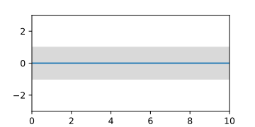
  A priori Gaussian process , represented by the expected value function and the area of ​​the confidence interval.

• 

  A posteriori Gaussian process with knowledge of three interpolation points, represented by random curves.

• 

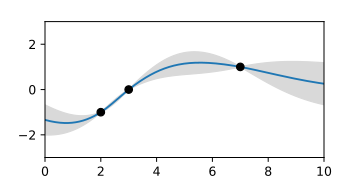
  A posteriori Gaussian process , represented by the expected value function and the area of ​​the confidence interval.

• 

  A posteriori Gaussian process with assumed measurement noise. The interpolations no longer hit the points exactly.

• 

  A posteriori Gaussian process with assumed measurement noise. The expected value becomes smoother and the confidence interval remains greater than zero.

• 

  A posteriori Gaussian process of interpolation of a gap, represented by the expected value function and the area of ​​the confidence interval

• 

  A posteriori Gaussian process of interpolating a gap, represented by animated random fluctuations according to the distribution.

The Python code of the examples can be found on the respective picture description page.

special cases

Undetermined readings

In some cases of conditional Gaussian processes, groups of linearly related measured values ​​are completely indeterminate, e.g. B. with indirect measured values ​​that follow from underdetermined equations, for example with a non-invertible positive semidefinite matrix of the form . The interpolation points then cannot simply be divided into known and unknown values ​​and the associated covariance matrix would be singular due to infinite uncertainties. That would correspond to a normal distribution which is infinitely extended in certain spatial directions transversely to the coordinate axes. In order to take into account the relationships between the indeterminate variables, the inverse matrix , the so-called precision matrix , must be used in such a case . This can describe completely indeterminate measured values, which is expressed by zeros in the diagonal. For such a distribution with partially unknown measured values and singular measurement uncertainties , the a posteriori distribution sought is calculated through the overlap with the a priori Gaussian process model by multiplying the probability densities. The union of the two normal distributions ${\displaystyle A^{\top }\Sigma ^{-1}A}$ ${\displaystyle \Sigma _{\text{2}}^{-1}}$ ${\displaystyle {\mathcal {N}}\left(\mu _{\text{2}},\Sigma _{\text{2}}\right)}$ ${\displaystyle \mu _{\text{2}}}$ ${\displaystyle \Sigma _{\text{2}}}$ ${\displaystyle {\mathcal {N}}\left(\mu _{\text{1}},\Sigma _{\text{1}}\right)}$

${\displaystyle \Sigma _{\text{Fusion}}=\left(\mathbb {I} +\Sigma _{\text{1}}\Sigma _{\text{2}}^{-1}\right)^{-1}\Sigma _{\text{1}}}$

${\displaystyle \mu _{\text{Fusion}}=\left(\mathbb {I} +\Sigma _{\text{1}}\Sigma _{\text{2}}^{-1}\right)^{-1}\mu _{\text{1}}+\Sigma _{\text{Fusion}}\Sigma _{\text{2}}^{-1}\mu _{\text{2}}}$

According to Operation Fusion, there is always a finite normal distribution, since one of the two is finite. If both input distributions are finite, then the result is identical to the a posteriori distribution, which is obtained with the formula for the conditional distribution.

Linear combination to a Gaussian process

A linear combination is to be formed from given basic functions , which has a maximum overlap with the distribution of an associated Gaussian process . Or measured values ​​are to be approximated while the interference signal contained therein is ignored as far as possible. In both cases, the coefficients searched for can be obtained using generalized least squares estimation ${\displaystyle \varphi _{j}(t)}$ ${\displaystyle {\mathcal {N}}(\mu ,\Sigma )}$ ${\displaystyle {\mathcal {GP}}(m,k)}$ ${\displaystyle \mu }$ ${\displaystyle {\mathcal {N}}(0,\Sigma )}$

${\displaystyle c=\left(A^{\top }\Sigma ^{-1}A\right)^{-1}A^{\top }\Sigma ^{-1}\mu }$

${\displaystyle \Sigma _{c}=\left(A^{\top }\Sigma ^{-1}A\right)^{-1}}$

be calculated. The matrix contains the function values ​​of the basic functions at the support points . The resulting coefficients c with the associated covariance matrix describe the linear combination with the greatest possible probability density in the distribution . The linear combination approximates the expected value function or the measured values in such a way that the residuals are best described by the covariance matrix . The method is used, for example, in the Scikit-learn program library to empirically estimate a polynomial expected value function of a Gaussian process. ${\displaystyle A_{ij}=\varphi _{j}(t_{i})}$ ${\displaystyle \varphi _{j}(t)}$ ${\displaystyle t_{i}}$ ${\displaystyle \Sigma _{c}}$ ${\displaystyle {\mathcal {N}}(\mu ,\Sigma )}$ ${\displaystyle \mu }$ ${\displaystyle \Sigma }$

Approximation of an empirical Gaussian process

A Gaussian process determined empirically from example functions ${\displaystyle f_{p}(t)}$

${\displaystyle m(t)={\frac {1}{N}}\sum _{p=1}^{N}f_{p}(t)}$

${\displaystyle k(t,t')={\frac {1}{N-1}}\sum _{p=1}^{N}\left[f_{p}(t)-m(t)\right]\cdot \left[f_{p}(t')-m(t')\right]}$

with a few strongly pronounced degrees of freedom can by means of an eigenvalue decomposition or the singular value decomposition

${\displaystyle \Sigma =VSV^{\top }}$

the covariance matrix can be approximated and simplified. To do this, one selects the largest eigenvalues ​​or singular values from the diagonal matrix . The associated columns of are the main components of the Gaussian process (see Principal Component Analysis ). If the columns are represented as functions , then the original Gaussian process is created by the mean value function and the covariance function ${\displaystyle \Sigma _{ij}=k(t_{i},t_{j})}$ ${\displaystyle n}$ ${\displaystyle \lambda _{p}=\sigma _{p}^{2}}$ ${\displaystyle S}$ ${\displaystyle v_{p}}$ ${\displaystyle V}$ ${\displaystyle v_{p}(t)}$ ${\displaystyle m(t)}$

${\displaystyle k(t,t')\approx \sum _{p=1}^{n}\sigma _{p}^{2}v_{p}(t)v_{p}(t')}$

approximated. This Gaussian process only describes functions of the linear combination

${\displaystyle f(t)=m(t)+\sum _{p}c_{p}v_{p}(t)}$,

where each coefficient is spread around the mean value zero as an independent random variable of the variance . ${\displaystyle c_{p}}$ ${\displaystyle \sigma _{p}^{2}=\lambda _{p}}$

Such a simplification is positively semidefinite and it usually lacks the properties for describing small-scale variations. These properties can be added to the covariance function in the form of a residual fitted stationary covariance function:

${\displaystyle k(t,t')\approx \sum _{p=1}^{n}\sigma _{p}^{2}v_{p}(t)v_{p}(t')+k_{\text{stat}}(t'-t)}$

Temporal Gauss-Markov process

In the case of covariance functions with a large number of spatial and temporal support points, very large and computationally intensive covariance matrices can arise. If, in such a case, the stationary time dependence can be described using the Gauss-Markov process (exponentially decreasing covariance function), then the estimation problem can be efficiently solved by an iterative approach using the Kalman filter .

Application examples

Example: trend forecast

In an application example from market research, the future demand for the topic of "snowboards" is to be predicted. For this purpose, an extrapolation of the number of Google search queries for this term should be calculated.

In the past data one recognizes a periodic, but not sinusoidal season dependence, which can be explained by the winter in the northern hemisphere. In addition, the trend has steadily decreased over the past decade. In addition, there is a recurring increase in search queries during the Olympic Games every four years. The covariance function was therefore modeled with a slow trend and a one- and four-year period:

${\displaystyle k(r)=0.8\exp \left(-{\tfrac {1}{2}}\left|\sin(\pi r)\right|-|r/25|^{2}-2.5\right)+(0.2-0.01)\exp \left(-\left|\sin \left({\tfrac {1}{4}}\pi r\right)\right|/0.2\right)+0.01\exp \left(-r/45\right)}$

The trend seems to show a clear asymmetry, which can be the case if the underlying random effects do not add up but reinforce each other, which results in a log-normal distribution . However, the logarithm of such values ​​describes a normal distribution to which Gaussian regression can be applied.

The figure shows an extrapolation of the curve (to the right of the dashed line). Since the results here were transformed back from the logarithmic representation using an exponential function, the predicted confidence intervals are correspondingly asymmetrical (gray area). The extrapolation shows the seasonal trends very plausibly and even predicts an increase in search queries for the Olympic Games.

This example with mixed properties clearly shows the universality of Gaussian regression compared to other interpolation methods, which are mostly optimized for special properties.

Python source code of the sample calculation

Example: sensor calibration

In an application example from industry, sensors are to be calibrated with the help of Gaussian processes. Due to manufacturing tolerances, the characteristics of the sensors show large individual differences. This causes high calibration costs, since a complete characteristic curve would have to be measured for each sensor. However, the effort can be minimized by learning the exact behavior of the scattering using a Gaussian process. For this purpose, the complete characteristic curves are measured by randomly selected representative sensors and thus the Gaussian process of scattering ${\displaystyle f(x)}$ ${\displaystyle N}$ ${\displaystyle f_{i}(x)}$ ${\displaystyle {\mathcal {GP}}(m,k)}$

${\displaystyle m(x)={\frac {1}{N}}\sum _{i=1}^{N}f_{i}(x)}$

${\displaystyle k(x,x')={\frac {1}{N-1}}\sum _{i=1}^{N}\left[f_{i}(x)-m(x)\right]\cdot \left[f_{i}(x')-m(x')\right]}$

calculated. In the example shown, 15 representative characteristics are given. The resulting Gaussian process is represented by the mean value function and the confidence interval. ${\displaystyle m(x)}$ ${\displaystyle m(x)\pm {\sqrt {k(x,x)}}}$

With the conditional Gaussian process with ${\displaystyle {\mathcal {GP}}(m_{\text{post}},k_{\text{post}})}$

${\displaystyle m_{\mathrm {post} }(x)=m(x)+\mathbf {k} ^{\top }(x,\mathbf {x} )K(\mathbf {x} ,\mathbf {x} )^{-1}(\mathbf {y} -m(\mathbf {x} ))}$

${\displaystyle k_{\mathrm {post} }(x,x')=k(x,x')-\mathbf {k} ^{\top }(x,\mathbf {x} )K(\mathbf {x} ,\mathbf {x} )^{-1}\mathbf {k} (\mathbf {x} ,x')}$

the complete map can now be reconstructed for each new sensor with a few individual measured values at the coordinates . The number of measured values ​​must correspond at least to the number of degrees of freedom of the tolerances that have an independent linear influence on the shape of the characteristic curve. ${\displaystyle \mathbf {y} }$ ${\displaystyle \mathbf {x} }$

In the example shown, a single measured value is not enough to clearly and precisely determine the characteristic. The confidence interval shows the area of ​​the curve that is not yet sufficiently accurate. With another measured value in this range, the remaining uncertainty can finally be completely eliminated. The sample fluctuations of the very differently acting sensors in this example seem to be caused by the tolerances of only two relevant internal degrees of freedom.

Python source code of the sample calculation

Example: signal decomposition

In an application example from signal processing, a time signal is to be broken down into its components. Let it be known about the system that the signal consists of three components, the three covariance functions

${\displaystyle k_{1}(r)=2.7^{2}\exp(-r^{2})}$

${\displaystyle k_{2}(r)=2.7^{2}\exp(-0.4|\sin(r/2.5)|)}$

${\displaystyle k_{3}(r)=0.6^{2}\delta _{r}}$

consequences. The sum signal then follows the covariance function according to the addition rule

${\displaystyle k_{\text{sum}}(r)=k_{1}(r)+k_{2}(r)+k_{3}(r)}$.

The following two figures show three random signals that were generated and added with these covariance functions for demonstration purposes. In the sum of the signals, the periodic signal hidden in it can hardly be seen with the naked eye, since its spectral range overlaps that of the other two components.

• 

  Individual signals : Three randomly generated signals that follow specific Gaussian processes.

• 

  Sum : The sum of the three signals.

With the help of the operation decomposition , the sum can be broken down into the three components ${\displaystyle y_{\text{sum}}}$

${\displaystyle y_{1}=\Sigma _{1}\Sigma _{\text{sum}}^{-1}y_{\text{sum}}+3}$

${\displaystyle y_{2}=\Sigma _{2}\Sigma _{\text{sum}}^{-1}y_{\text{sum}}-3}$

${\displaystyle y_{3}=\Sigma _{3}\Sigma _{\text{sum}}^{-1}y_{\text{sum}}}$

be disassembled, with . The estimate of the most likely decomposition shows how well the separation is possible in this case and how close the signals are to the original signals. The estimated uncertainties, taking into account the cross-correlations, are shown in the animation by random fluctuations. ${\displaystyle (\Sigma _{x})_{ij}=k_{x}(|t_{j}-t_{i}|)}$

• 

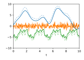
  Decomposition : Most likely decomposition given knowledge of the respective covariance functions. The original signals are shown in dashed lines.

• 

  Uncertainty : Estimated uncertainties represented by animated random fluctuations according to the (cross) covariance matrices.

The example shows how very different types of signals can be separated in one step with this method. Other filter methods such as sliding averaging, Fourier filtering, polynomial regression or spline approximation, on the other hand, are optimized for special signal properties and provide neither precise error estimates nor cross-correlations.

If the Gaussian processes of the individual components are not exactly known for a given signal, then in some cases a hypothesis test can be carried out with the aid of the log-marginal likelihood function, provided that sufficient data is available for good conditioning of the function. The parameters of the assumed covariance functions can be adapted to the measurement data by maximizing them.

Python source code of the sample calculation

literature

• CE Rasmussen, Gaussian Processes in Machine Learning doi : 10.1007 / 978-3-540-28650-9_4 ( pdf ), Advanced Lectures on Machine Learning. ML 2003. Lecture Notes in Computer Science, vol 3176. Springer, Berlin, Heidelberg
• CE Rasmussen, CKI Williams, Gaussian Processes for Machine Learning ( pdf ), MIT Press , 2006. ISBN 0-262-18253-X .
• RM Dudley, Real Analysis and Probability , Wadsworth and Brooks / Cole, 1989.
• B. Simon, Functional Integration and Quantum Physics , Academic Press, 1979.
• ML Stein, Interpolation of Spatial Data: Some Theory for Kriging , Springer, 1999

Web links

Teaching material

• Gaussian Processes Web Site (textbook, tutorials, code etc.)
• Interactive Gaussian Regression Demo
• The Kernel Cookbook (Guide to Constructing Covariance Functions)

software

• GPy - A Gaussian processes framework in Python
• Scikit Learn Gaussian Process - Gaussian process module of the machine learning library Scikit-learn for Python
• ooDACE - A flexible Matlab toolbox.
• GPstuff - Gaussian process toolbox for Matlab and Octave
• Gaussian process library written in C ++ 11

Individual evidence

1. ↑ Rasmussen / Williams: Gaussian Processes for Machine Learning , see Chapter 4.2.2 Dot Product Covariance Functions , page 89 and Table 4.1, page 94.
2. ↑ Rasmussen / Williams: Gaussian Processes for Machine Learning , see Chapter 4 Covariance Functions , valid covariance functions are listed, for example, in Table 4.1 on page 94 as ND .
3. ↑ The general linear transformation is derived from the equation by choosing the matrix F as [AB], as a vector ( ) and from the corresponding four blocks. ${\displaystyle F\cdot {\mathcal {N}}\left(\mu ,\Sigma \right)={\mathcal {N}}\left(F\mu ,F\Sigma F^{\top }\right)}$ ${\displaystyle \mu }$ ${\displaystyle \mu _{1}}$ ${\displaystyle \mu _{2}}$ ${\displaystyle \Sigma }$
4. ↑ The derivation is based on the covariance rule for multiplication and associativity . ${\displaystyle {\text{cov}}(Ax,By)=A{\text{cov}}(x,y)B^{\top }}$ ${\displaystyle {\text{cov}}(x,y+z)={\text{cov}}(x,y)+{\text{cov}}(x,z)}$
5. ↑ Rasmussen / Williams: Gaussian Processes for Machine Learning , see Chapter 4.2.4 Making New Kernels from Old , page 94.
6. ↑ Rasmussen / Williams: Gaussian Processes for Machine Learning , see Chapter 5.2 Bayesian Model Selection , page 94.
7. ↑ The data is available from Google Trends using the search term "snowboard" .
8. ↑ With stationary Gaussian processes: Tao Chen et al .: Calibration of Spectroscopic Sensors with Gaussian Process and Variable Selection , IFAC Proceedings Volumes (2007), Volume 40, Issue 5, DOI: 10.3182 / 20070606-3-MX-2915.00141
9. ↑ Honicky, R. "Automatic calibration of sensor-phones using gaussian processes." EECS Department, UC Berkeley, Tech. Rep. UCB / EECS-2007-34 (2007), pdf