Wiener Trial

Two example paths of a standard Wiener process

A Wiener process (after the US mathematician Norbert Wiener ) is a time-continuous stochastic process that has normally distributed , independent increases . It represents a mathematical model for the Brownian movement and is therefore often referred to as “Brownian movement”.

Since the introduction of stochastic analysis by Itō Kiyoshi in the 1940s, the Wiener process has played the central role in the calculation of time-continuous stochastic processes and in many areas of natural and economic sciences it serves as the basis for modeling random developments.

history

Thorvald N. Thiele

Louis Bachelier

In 1827 the Scottish botanist Robert Brown observed under the microscope how plants pollen moved irregularly back and forth in a drop of water (hence the name Brownian movement ).

1880 described the statistician and astronomer Thorvald N. Thiele (1838-1910) in Copenhagen for the first time such a "process" (the theory of stochastic processes had not yet been developed) when he economic time series and the distribution of residuals in the method of least squares studied. In 1900, the French mathematician Louis Bachelier (1870-1946), a pupil of Henri Poincare , took up Thiele's idea when he was trying to analyze price movements on the Paris stock exchange . In the end, both approaches had little impact on the future development of the process, partly because financial mathematics played a subordinate role in mathematics at the time; today, however, it is considered the main area of ​​application for Viennese trials. Still preferred z. B. the stochastic William Feller called the Bachelier-Wiener process .

The breakthrough came when Albert Einstein in his annus mirabilis in 1905 , apparently without knowledge of Bachelier's work, and independently of him, Marian Smoluchowski defined the Vienna Trial in its present form in 1906. Einstein's motivation was to explain the movement of Brownian particles through the molecular structure of water - an approach that was extremely controversial at the time, but is now undisputed - and to support this explanation mathematically. Interestingly enough , he did not demand another, physically meaningful property, the rectifiability of the random paths , for his model. Although this means that the particles travel an infinitely long distance every second (which theoretically disqualifies the entire model), the Einsteinian approach meant the breakthrough for both molecular theory and the stochastic process.

Einstein, however, failed to provide any proof of the probabilistic existence of the process. This was not achieved until 1923 by the American mathematician Norbert Wiener , who was able to use new tools from Lebesgue and Borel in the field of measure theory . Yet its proof was so long and complicated that only a handful of contemporaries could understand it. Ito Kiyoshi is said to have made some of his greatest advances in the development of the stochastic integral while trying to understand Wiener's work.

Ultimately, it was Itō who paved the way for the Wiener process from physics to other sciences: the stochastic differential equations he established made it possible to adapt Brownian motion to more statistical problems. The geometric Brownian motion derived from a stochastic differential equation solves the problem that the Wiener process, regardless of its starting value, almost certainly reaches negative values ​​in the course of time, which is impossible for stocks; Bachelier's approach ultimately failed because of this. Since the development of the famous Black-Scholes model , the geometric Brownian movement has therefore been the standard.

The problem raised by the non-rectifiable paths of the Wiener process in the modeling of Brownian paths leads to the Ornstein-Uhlenbeck process and also makes clear the need for a theory of stochastic integration and differentiation - here it is not the motion, but the speed of the particle that is considered as one Modeled a rectifiable process derived from the Wiener process, from which rectifiable particle paths are obtained through integration.

Today, in practically all natural and many social sciences, Brownian movements and related processes are used as tools.

definition

A Wiener process is a time-continuous stochastic process that has normally distributed , independent increases:
A stochastic process on the probability space is called a (standard) Wiener process if the following four conditions apply: ${\displaystyle (W_{t})_{t\in \mathbb {R} _{+}}}$ ${\displaystyle (\Omega ,{\mathcal {A}},P)}$

1. ${\displaystyle W_{0}=0}$(P- almost certainly ).
2. For given points in time , the increases are stochastically independent . The Vienna Process thus has independent gains. ${\displaystyle 0\leq t_{0}<t_{1}<t_{2}<\dotsb <t_{m}}$ ${\displaystyle W_{t_{1}}-W_{t_{0}},W_{t_{2}}-W_{t_{1}},\dotsc ,W_{t_{m}}-W_{t_{m-1}}}$
3. For all true . The increases are therefore stationary and normally distributed with the expected value zero and the variance . ${\displaystyle 0\leq s<t}$ ${\displaystyle W_{t}-W_{s}\;\sim \;{\mathcal {N}}\left(0,t-s\right)}$ ${\displaystyle t-s}$
4. The individual paths are (P-) almost certainly continuous .

The fourth point can also be deleted from the definition insofar as it can be shown with the continuity theorem of Kolmogorow-Tschenzow that under the above There is always an almost certainly steady version of the process .

Alternatively, a Wiener process according to Paul Lévy can be characterized by the following two properties: ${\displaystyle (W_{t})_{t\in \mathbb {R} _{+}}}$

1. ${\displaystyle W_{t}}$is a steady local martingale with . ${\displaystyle W_{0}=0}$
2. ${\displaystyle {W_{t}}^{2}-t}$ is a martingale.

properties

classification

• The Wiener process belongs to the family of the Markov processes and there specifically to the class of the Levy processes . He also fulfills the strong Markov quality .
• The Wiener process is a special Gaussian process with an expected value function and a covariance function . ${\displaystyle \operatorname {E} (W_{t})=0}$ ${\displaystyle \operatorname {Cov} (W_{s},W_{t})=\min(s,t)}$
• The Vienna Trial is a martingale . So if the filtration produced by , then the conditional expectation applies to all . ${\displaystyle ({\mathcal {F}}_{t})_{t\geq 0}}$ ${\displaystyle (W_{t})_{t\geq 0}}$ ${\displaystyle E(W_{t}\mid {\mathcal {F}}_{s})=W_{s}}$ ${\displaystyle 0\leq s<t}$
• The Wiener process is a Lévy process with continuous paths and constant expected value . ${\displaystyle 0}$

Properties of the paths

• The paths of a Viennese trial are almost certainly not differentiable at any point ( theorem of Paley-Wiener-Zygmund ) and almost certainly not rectifiable .
• The paths almost certainly have infinite variation in each interval . ${\displaystyle [s,t]\subset \mathbb {R} _{+}}$
• For the quadratic variation it is almost certain . ${\displaystyle [W,W]_{t}=\langle W,W\rangle _{t}=t}$
• The laws of the iterated logarithm provide information about asymptotics at infinity and around the zero point .
• The following applies to a Viennese trial ${\displaystyle (W_{t})_{t\geq 0}}$

${\displaystyle \limsup _{h\rightarrow 0}\left({\frac {\sup _{t\in [0,h]}|W_{t+h}-W_{t}|}{(2h\log({\frac {1}{h}}))^{\frac {1}{2}}}}\right)=1}$

pretty sure. Thus, the paths of the Wiener process are especially Hölder-continuous to the exponent with , but not for . ${\displaystyle \alpha }$ ${\displaystyle \alpha <{\frac {1}{2}}}$ ${\displaystyle \alpha ={\frac {1}{2}}}$

Self-similarities, principle of reflection

• Also the negative of a standard Wiener process, so it is a standard Wiener process. The principle of reflection also applies more generally : a Wiener process mirrored at any given stopping time is again a Wiener process. The mirrored process is defined as follows: if and if . ${\displaystyle (-W_{t}),\;t\geq 0,}$ ${\displaystyle \tau }$ ${\displaystyle {\hat {W}}_{t}}$ ${\displaystyle {\hat {W}}_{t}(\omega )=W_{t}(\omega )}$ ${\displaystyle t\leq \tau (\omega )}$ ${\displaystyle {\hat {W}}_{t}(\omega )=2W_{\tau (\omega )}(\omega )-W_{t}(\omega )}$ ${\displaystyle t>\,\tau (\omega )}$
• The Wiener process is self-similar , stretching the time axis, i.e. H. is a standard Viennese process for everyone. ${\displaystyle X_{t}={\tfrac {1}{\sqrt {\alpha }}}\cdot W_{\alpha \cdot t}}$ ${\displaystyle \alpha >0}$
• Inversion of the time axis: also is a standard Wiener process ${\displaystyle X_{t}=tW_{\frac {1}{t}}}$
• Shifting the time axis: for every deterministic process , the stochastic process is also a Wiener process; here the increases are considered from the point in time , i. H. fulfills the weak Markov property. ${\displaystyle s\geq 0}$ ${\displaystyle X_{t}=W_{t+s}-W_{s}}$ ${\displaystyle s}$ ${\displaystyle W}$

generator

A brownish movement on the sphere. The generator of this process is ½ times the Laplace-Beltrami operator on a manifold, here a spherical surface.

The following applies to the generator of a one-dimensional standard Wiener process ${\displaystyle A}$

${\displaystyle Af(x)=\lim \limits _{t\downarrow 0}{\frac {E(f(x+W_{t}))-f(x)}{t}}={\frac {1}{2}}f''(x)}$,

that is , ½ times the operator of the second derivative. More generally, the generator of a multi-dimensional Wiener process is ½ times the Laplace operator . This relationship can be used to refer to Wiener processes on other manifolds such as B. on a sphere (see picture), namely as a Markov process with the Laplace-Beltrami operator as a generator. ${\displaystyle A}$

Generalized Wiener process

If a standard Wiener process is called the stochastic process ${\displaystyle (W_{t})}$

${\displaystyle X_{t}=\mu t+\sigma W_{t}}$

Brownian motion with drift and volatility . This also enables stochastic processes to be represented that tend to fall ( ) or tend to rise ( ). The following applies ${\displaystyle \mu }$ ${\displaystyle \sigma }$ ${\displaystyle \mu <0}$ ${\displaystyle \mu >0}$

${\displaystyle X_{t}-X_{s}\sim {\mathcal {N}}\left(\mu (t-s),\sigma ^{2}\left(t-s\right)\right)}$.

General Wiener processes are also Markov and Lévy processes, but the martingale property is only valid in a weakened form:

Is so is a super martingale , is so is a submartingale . For is a martingale . ${\displaystyle \mu \leq 0}$ ${\displaystyle X_{t}}$ ${\displaystyle \mu \geq 0}$ ${\displaystyle X_{t}}$ ${\displaystyle \mu =0}$ ${\displaystyle X_{t}}$

The multi-dimensional case

75 steps of a discrete approximation to a two-dimensional Brownian movement. The particle could have moved in a similar way under Brown's microscope.

A multi-dimensional stochastic process is called an n-dimensional (standard) Wiener process or n-dimensional Brownian motion if the coordinates are independent (standard) Wiener processes. The increases are then also independent and distributed ( n-dimensional normal distribution ), where the unit matrix of dimension is n . ${\displaystyle W_{t}=(W_{1,t},W_{2,t},\ldots W_{n,t})^{T},\;t\geq 0}$ ${\displaystyle (W_{i,t})}$ ${\displaystyle W_{t}-W_{s}}$ ${\displaystyle {\mathcal {N}}(0,(t-s)I_{n})}$ ${\displaystyle I_{n}}$

The n-dimensional Wiener process has a particularly beautiful property that sets it apart from most other multi-dimensional processes and that predestines it for modeling the Brownian particle: it is invariant when the coordinate axes are rotated. This means that for every orthogonal matrix the rotated (or mirrored) process has exactly the same distribution as . ${\displaystyle Q\in \mathbb {R} ^{n\times n}}$ ${\displaystyle X_{t}:=QW_{t},\;t\geq 0}$ ${\displaystyle W_{t}}$

Just like the one-dimensional Brownian motion, one can now generalize the n-dimensional motion: For every vector and every matrix , is through ${\displaystyle \mu \in \mathbb {R} ^{n}}$ ${\displaystyle A\in \mathbb {R} ^{n\times n}}$

${\displaystyle X_{t}:=\mu t+AW_{t},\;t\geq 0}$

defines a Brownian motion with drift and variance . The following applies accordingly . The individual coordinates can thus also be correlated with one another . ${\displaystyle \mu }$ ${\displaystyle AA^{T}}$ ${\displaystyle X_{t}\sim {\mathcal {N}}(\mu t,tAA^{T})}$

Relationship to other stochastic processes

• If there is a geometric Brownian movement , then it is a Brownian movement (with drift). On the other hand, one can gain from any Viennese process with drift and volatility through a geometric Brownian movement. ${\displaystyle (X_{t})_{t\geq 0}}$ ${\displaystyle W_{t}:=\ln(X_{t})}$ ${\displaystyle (X_{t})_{t\geq 0}}$ ${\displaystyle \mu }$ ${\displaystyle \sigma }$ ${\displaystyle Y_{t}:=e^{X_{t}-{\frac {\sigma ^{2}t}{2}}}}$
• With the help of Itô's stochastic integral term, the Wiener process can be generalized to the Itō process .
• The symmetric random walk can be considered a discrete-time equivalent of the Wiener process, because it is the following convergence theorem: for the random walk on the discrete time grid defined so that valid and in each time step with probability to upward and likely to down moves, then converges for against a standard Wiener process (Donsker's principle of invariance). ${\displaystyle n\in \mathbb {N} }$ ${\displaystyle (R_{t})_{t\in T}}$ ${\displaystyle T=\left\{0,{\tfrac {1}{n}},{\tfrac {2}{n}},\ldots \right\}}$ ${\displaystyle R_{0}=0}$ ${\displaystyle R}$ ${\displaystyle 1/2}$ ${\displaystyle {\sqrt {\tfrac {1}{n}}}}$ ${\displaystyle 1/2}$ ${\displaystyle {\sqrt {\tfrac {1}{n}}}}$ ${\displaystyle R}$ ${\displaystyle n\to \infty }$
• If and is a standard Viennese process , then is a Brownian bridge . ${\displaystyle (W_{t})_{t\geq 0}}$ ${\displaystyle T>0}$ ${\displaystyle B_{t}:=W_{t}-{\tfrac {t}{T}}W_{T},\ 0\leq t\leq T}$

Simulation of Brownian paths

Various methods are available to simulate paths of a Wiener process with the help of random numbers , all of which are based on different properties of the process:

Simple random walk

The simplest possibility is to use the above-mentioned convergence of the simple random walk against a Wiener process. To do this, one only has to simulate random variables B ₁ , B ₂ , B ₃ , ... distributed by Rademacher , which are independent of one another and each with a probability of taking the values ​​1 and −1. Then one can at a predetermined pitch a Wiener process at the locations by ${\displaystyle {\tfrac {1}{2}}}$ ${\displaystyle \Delta t\geq 0}$ ${\displaystyle 0,\;\Delta t,\;2\,\Delta t,\;3\,\Delta t\ldots }$

${\displaystyle W_{n\Delta t}\approx {\sqrt {\Delta t}}\sum _{i=1}^{n}B_{i}}$

approximate. The advantage of this method is that only rademacher-distributed random variables that are very easy to produce are required. However, it is only an approximation: the result is not a Gaussian process, but has quasi binomially distributed states (more precisely, it is binomially (n; 0.5) -distributed). In order to approximate the normal distribution sufficiently well, the choice must therefore be very small. This method is therefore only recommended if you want to simulate the process on a very fine time grid anyway. ${\displaystyle {\frac {1}{2}}\left(\sum _{i=1}^{n}B_{i}+n\right)}$ ${\displaystyle \Delta t}$

Gaussian Random Walk

The following method is superior to the simple random walk (unless a particularly fine time grid is required), since it simulates the process exactly (i.e. the resulting states have the same distribution as those of a Wiener process):

${\displaystyle W_{n\Delta t}\approx {\sqrt {\Delta t}}\sum _{i=1}^{n}Z_{i}}$,

where are independent, standard normally distributed random numbers (for example generated by the Polar method of Marsaglia ). This discretization, known as Gaussian random walk , is only disadvantageous if the normally distributed random variables present are not of uniform “quality”. For example, when using quasi-random numbers , late-occurring numbers sometimes have dependency structures that can skew the result. In such a case, one of the following methods is preferable: ${\displaystyle Z_{1},\;Z_{2},\;Z_{3}\ldots }$

Brownian bridge

The first five halving steps of Brown's bridge, the newly simulated iteration is shown in red.

This method, which can be traced back to Paul Lévy (which only marginally has something to do with the stochastic process of the Brownian bridge ), uses the covariance structure of the Wiener process and places greater emphasis on early standard normal random variables . ${\displaystyle Z_{1},Z_{2},\ldots }$

First , which is normally distributed with variance 1 is simulated by. Now the interval is halved step by step and the following step is repeated: ${\displaystyle W_{1}}$ ${\displaystyle W_{1}=Z_{1}}$ ${\displaystyle [0,1]}$

${\displaystyle W_{\frac {1}{2}}}$results as the arithmetic mean plus a further normally distributed random variable to correct the variance. So: ${\displaystyle {\frac {1}{2}}(W_{0}+W_{1})}$

${\displaystyle W_{\frac {1}{2}}={\frac {1}{2}}(W_{0}+W_{1})+{\frac {1}{2}}Z_{2}}$

Analogous:

${\displaystyle {\begin{aligned}W_{\frac {1}{4}}&={\frac {1}{2}}(W_{0}+W_{\frac {1}{2}})+{\frac {1}{\sqrt {8}}}Z_{3}\\W_{\frac {3}{4}}&={\frac {1}{2}}(W_{\frac {1}{2}}+W_{1})+{\frac {1}{\sqrt {8}}}Z_{4}\\W_{\frac {1}{8}}&={\frac {1}{2}}(W_{0}+W_{\frac {1}{4}})+{\frac {1}{4}}Z_{5}\end{aligned}}}$

and so on. The factors are reduced by the factor in each halving step and ensure that the states receive the correct variance. ${\displaystyle {\tfrac {1}{2}},\;{\tfrac {1}{\sqrt {8}}},\;{\tfrac {1}{4}}\ldots }$ ${\displaystyle {\sqrt {2}}}$

In order to extend a Wiener process to an arbitrary interval , one can now apply the transformation described above ; is then a Viennese trial . ${\displaystyle [0,1]}$ ${\displaystyle [0,a]}$ ${\displaystyle X_{t}={\sqrt {a}}W_{\frac {t}{a}}}$ ${\displaystyle X}$ ${\displaystyle [0,a]}$

The background to this non-causal modeling is that it is conditionally distributed on and again normally. ${\displaystyle W_{(t_{0}+t_{1})/2}}$ ${\displaystyle W_{t_{0}}}$ ${\displaystyle W_{t_{1}}}$

Spectral decomposition

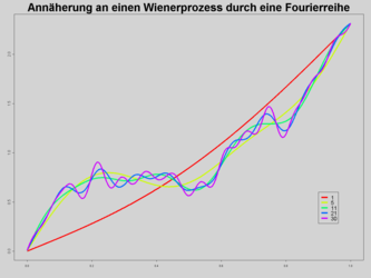
With the spectral decomposition, the Wiener process is approximated in a kind of stochastic Fourier analysis as trigonometric polynomials with random coefficients. If they are independent and standard normal distributed, then the series converges ${\displaystyle Z_{0},\;Z_{1},\;Z_{2}\ldots }$

${\displaystyle S(t)=Z_{0}\cdot t+\sum _{k=1}^{\infty }Z_{k}~{\frac {{\sqrt {2}}\cdot \sin(k\pi t)}{k\pi }}}$

against a Viennese trial. This method converges with maximum speed with regard to the L ² norm , but, in contrast to the Brownian bridge, contains many complex trigonometric function evaluations. Therefore it is used less often , especially in the Monte Carlo simulation .

• Approach to a Wiener process by means of a Fourier series
• 
• 

geometry

The one- and two- dimensional Brownian movement is recurrent , in all higher dimensions it is transient . ( Sentence by Pólya (random walks) : “A drunk man always finds his way home, a drunken bird doesn't.”) See also Markow chain .

literature

• Andrei N. Borodin, Paavo Salminen: Handbook of Brownian Motion - Facts and Formulas. Birkhäuser, Basel 2002, ISBN 3-7643-6705-9 .
• Ioannis Karatzas, Steven E. Shreve: Brownian Motion and Stochastic Calculus (Graduate Texts in Mathematics). Springer, New York 1997, ISBN 0-3879-7655-8 .
• David Meintrup, Stefan Schäffler: Stochastics. Theory and applications. Springer, Berlin / Heidelberg 2005, ISBN 3-540-21676-6 , chap. 12, pp. 341-374.
• René L. Schilling, Lothar Partzsch: Brownian Motion. An Introduction to Stochastic Processes. De Gruyter, Berlin / Boston 2012, ISBN 978-3-11-027889-7 .
• John Michael Steele: Stochastic Calculus and Financial Applications. Springer, New York 2000, ISBN 0-387-95016-8 .

See also

• Broken Brownian movement
• Root diffusion process

Individual evidence

1. ↑ Einstein, Albert: About the motion of particles suspended in liquids at rest, required by the molecular kinetic theory of heat. In: Annals of Physics . tape 17 , 1905, pp. 549-560 .
2. ↑ Smoluchowski, M .: On the kinetic theory of Brownian molecular motion and suspensions . In: Annals of Physics . tape 21 , 1906, pp. 756-780 .
3. ↑ P. Lévy: Processus stochastiques et mouvement brownien. Gauthier-Villars, Paris 1965.