Scaling (computer graphics)

Raster graphics in original size

Raster graphics after double enlargement by means of pixel repetition

In computer graphics and digital image processing , scaling (from Italian scala , German "stairs") describes the change in size of a digital image . In video technology the increase of digital material as is up-scaling (upscaling) or Resolution Enhancement designated.

When scaling a vector graphic, the graphic primitives that make up the vector graphic are stretched through geometric transformation before rasterization , which does not cause any loss of image quality.

When raster graphics are scaled, their image resolution is changed. This means that a new image with a higher or lower number of image points ( pixels ) is generated from a given raster graphic . When the number of pixels is increased (upscaling), this is usually associated with a visible loss of quality. From the standpoint of digital signal processing , the scaling of raster graphics is an example of sample rate conversion , the conversion of a discrete signal from one sample rate (here the local sample rate) to another.

Applications

The scaling of images is used, among other things, in web browsers , image processing programs , image and file viewers , software magnifiers , with digital zoom , section enlargement and generation of preview images as well as with the output of images on screens or printers.

The enlargement of images is also important for the home theater sector , in which HDTV -capable output devices with material in PAL resolution, z. B. comes from a DVD player . The upscaling is carried out in real time by special chips (video scaler) , whereby the output signal is not saved. The upscaling is in contrast to the up- converting of a material, in which the output signal does not necessarily have to be created in real time, but is saved for this.

Scaling methods for raster graphics

Scaling with reconstruction filter

Image editing programs usually offer several scaling methods. The most commonly supported methods - pixel repetition, bilinear and bicubic interpolation - scale the image using a reconstruction filter .

When scaling, the specified image grid must be transferred to an output grid of different sizes. The scaling can therefore be clearly represented by placing the pixel grid of the output image to be calculated over the pixel grid of the input image. Each pixel of the output image is assigned a color value that is calculated from the pixels of the input image that are in the vicinity. The reconstruction filter used determines which pixels of the input image are used for the calculation and how their color values are weighted.

Enlargement of a 6 × 6 pixel raster graphic to 11 × 11 pixels (the lower image resolutions in this example were chosen for better clarity; the principle is the same for higher resolutions).

1) input image; the pixels are shown here as circles.
2) The pixel grid of the output image, shown here as yellow crosses, is placed over the input image.
3) The color values of the output image are calculated from the nearby pixels of the input image.
4) output image.

Scaling using a radially symmetrical reconstruction filter (carrier shown in green). A color value of the output image is calculated as the sum of color values of the input image weighted by the reconstruction filter.

When scaling, a two-dimensional reconstruction filter is placed over each pixel of the output image. The color value is calculated as the sum of the color values of the pixels of the input image that are overlapped by the carrier of the reconstruction filter, weighted by the value of the reconstruction filter at these pixels.

Usually, reconstruction filters decrease with increasing distance from the center. As a result, color values located close to the output pixel are weighted more heavily and those further away are weighted less. The size of a reconstruction filter is based on the raster of the input image and, in the case of reduction, on the raster of the output image.

Some reconstruction filters have negative partial areas; Such filters lead to a sharpening of the image similar to unsharp masking . Color values outside the permitted range of values can arise, which are then usually set to the minimum or maximum value. In addition, it must be taken into account that fewer pixels are overlapped by the reconstruction filter at the image edges than in the rest of the image. In order to prevent dark pixels at the image edges, the filter must be renormalized here. The determined color value of the output image is divided by the sum of the values of the reconstruction filter at the overlapped pixels of the input value. Another possibility is to use the closest color value at the edge of the image for points falling outside the image.

Construction of two-dimensional filters

When comparing different reconstruction filters, the one-dimensional filters can first be considered. Reconstruction filters that are defined as polynomials are also called splines . Other known filters are the Lanczos filter and the Gaussian filter .

There are two ways in which a one-dimensional reconstruction filter can be generated from a two-dimensional one, namely through radial symmetry and through separation.

Construction through radial symmetry: A two-dimensional, radially symmetrical reconstruction filter can be generated as a surface of revolution of a one-dimensional filter. The filter value depends solely on the distance from the center. In order to apply radially symmetrical reconstruction filters, the Euclidean distance to the pixels of the input image must therefore be calculated. Radially symmetrical filters lead to sampling frequency ripple: when enlarging a monochrome area, the color values can vary from pixel to pixel, unless the filter is renormalized for each pixel.

Construction through separation: Most scaling methods use separable square-beam filters. In the case of separable filters, the calculation using a two-dimensional filter can be replaced by a series of interpolations with a one-dimensional reconstruction filter. Here, in an intermediate step, the interpolated point at the x -coordinate of the output pixel is calculated for each of the image lines overlapped by the filter . The interpolated color value at the output pixel is then calculated from the vertical points generated in this way.

Separable filters lead to anisotropy : Image artifacts that result from separable filters are not isotropically (evenly distributed in all directions), but are preferably aligned horizontally and vertically. Since only a sequence of one-dimensional interpolations has to be carried out with separable filters and no Euclidean distances are calculated, they can be calculated more quickly than radially symmetric filters.

The Gaussian filter is the only radially symmetrical reconstruction filter that is also separable. With all other filters, the separable and the radially symmetrical generation lead to different results.

Pixel repetition

With pixel repetition, also called nearest neighbor , the color value of the closest pixel of the input image is assigned to each pixel of the output image. Shrinking images with this method can lead to severe aliasing , which manifests itself as image artifacts. When enlarging by means of pixel repetition, there is a block-like, "pixelated" representation.

In the case of enlargement, the pixel repetition corresponds to the reconstruction with a 1 × 1 pixel box filter. Such a filter only overlaps one pixel of the input image, namely the closest one.

Enlargement through pixel repetition

Bilinear interpolation

When scaling using bilinear interpolation, a color value of the output image is calculated from the four closest color values of the input image.

With bilinear interpolation , the color value of a pixel in the output image is interpolated from the four neighboring color values in the input image.

This filter is separable and can be calculated as a series of interpolations with a one-dimensional reconstruction filter (the triangle filter). An interpolated color value is first calculated for each of the two picture lines involved, and then interpolation is carried out between these two vertical points. With this method, the color value of the output pixel is calculated as follows: ${\ displaystyle P (x, y)}$

{\ displaystyle Q_ {0} = (1-d_ {x}) P_ {00} + d_ {x} P_ {10}}

{\ displaystyle Q_ {1} = (1-d_ {x}) P_ {01} + d_ {x} P_ {11}}

{\ displaystyle P (x, y) = (1-d_ {y}) Q_ {0} + d_ {y} Q_ {1}}

The bilinear interpolation corresponds to the reconstruction with a filter of the functional equation for and in . ${\ displaystyle z = (1- | x |) (1- | y |)}$ ${\ displaystyle x}$ ${\ displaystyle y}$ ${\ displaystyle [-1.1]}$

Magnification through bilinear interpolation

Bicubic interpolation

With bicubic interpolation, a color value of the output image is interpolated from the neighboring color values of the input image using cubic splines (see Mitchell-Netravali filter ). There are several common cubic splines with different properties; the term “bicubic interpolation” is therefore ambiguous.

The image processing program GIMP (version 2.7) uses Catmull-Rom splines. With this spline type, the color values at edges overshoot , which manifests itself as a sharpening of the image. The image processing program Paint.NET (version 3.36), on the other hand, uses cubic B-splines, which lead to a more blurred representation. Also, Catmull-Rom splines are only - smooth , while cubic B splines are - smooth . ${\ displaystyle C ^ {1}}$ ${\ displaystyle C ^ {2}}$

Both GIMP and Paint.NET use the separable variant of the two-dimensional reconstruction filter with a 4 × 4 pixel carrier. As with bilinear interpolation, the two-dimensional filter can be replaced by a series of interpolations with a one-dimensional filter.

Enlargement with a separable Catmull-Rom filter

Magnification with a separable cubic B-spline filter

Other scaling methods

Example of enlargement using a super-resolution process. The left image shows an original image from a series of nine images, enlarged twice with pixel repetition. The right picture shows the result of a two-fold enlargement after combining the nine original pictures by SR.

Super resolution process: When scaling using so-called super-resolution (SR) methods, information from the neighboring images of a single image from a sequence is used. A higher quality is achieved with a higher computational effort. Such methods are particularly relevant for medicine, astrophotography and forensic analysis of recordings from surveillance cameras . These methods are also of interest for upscaling in the home theater area; simpler algorithms are used for such real-time applications.

There is also the single-image super-resolution method, which, through an analysis of sample images in different resolutions, determines statistical information that is used during scaling. Another technique is to detect repetitive details in the image in different sizes, which are then scaled based on the greatest detail.

Content-dependent image distortion: The content-dependent image distortion is a process with which the aspect ratios of images are changed while retaining the relevant image content.

Scaling of pixel art: Special algorithms have been developed for enlarging pixel art images with hard edges, which deliver better results than the methods described above for these image types. Some of these algorithms can scale images to two, three or four times their original size in real time, while others output vector graphics.

Scaling a pixel art image to 300% through pixel repetition
Scaling by the Hq3x algorithm

Non-linear scaling of vector graphics

Requirements for technical graphics

Technical drawings such as construction, building and surveying plans as well as maps contain symbols, dimensions and explanatory text entries in addition to the object geometry. These drawings are based on pure vector graphics and are therefore easy to influence. The design of these plans has been standardized by general and branch-specific drawing standards and sample sheets to such an extent that users can interpret and implement these plan contents. Serve as a means of uniform planning

Symbols for small-scale objects, point representation and standard components
Line patterns for different line types (e.g. hidden / visible)
Highlighting of important lines through enlarged line width
Area display using circumferential lines, hatching or colored areas
Dimensions with dimensional chains
Texts assigned to objects for special statements or information.

In the case of technical drawings, a good plan is important in order to interpret the plan content. This includes that the presentation of the essential plan content and the explanatory additional information are in a balanced relationship, which is only possible in the scaling range that meets these requirements. For output, vector graphics must be converted into raster graphics, the limits of which therefore also apply to vector graphics during output. Enlargements are generally less problematic, here the plan size limits the scaling. However, when reduced, fewer pixels are available for the same information density; the representation then quickly appears overloaded and is difficult to differentiate.

In the course of this conversion, however, it is possible to influence the output, for example to hide details that are too small and therefore indistinctly recognizable. In the case of symbol outputs, text entries and dimensions, the importance of the entry can generally be recognized by the size of the representation, which ensures a good overview, because the plan user gains an overall impression more easily and can better familiarize himself with the plan content. Subordinate details, on the other hand, are indicated by a small but still legible representation. This method of representation enables the information density to be controlled automatically to a certain extent.

Linear scaling issues

Each additional piece of information in a graphic requires a free area, because it should at most overlay and displace the primary object representation to such an extent that this gap in perception can be "jumped over". The information density of a plan thus determines the basic scale of the presentation. There are narrow limits to a reduction in size because texts and symbols below a certain size, around 1.3 mm, are no longer legible. Even enlargements cannot be made at will. Due to linear scaling, the additional information, deliberately cautiously presented in the basic plan, quickly becomes very dominant and thus significantly disrupts the overall impression. With a scaling by a factor of 2, the plane area occupied by symbols and texts grows by a square factor of 4 and is perceived more in the foreground. In the case of area hatching, on the other hand, the area impression of hatching lapses because the hatching spacing becomes too large and takes on the impression of parallel individual lines. The perception of the essential plan contents becomes more difficult due to too much additional information and results in a poorer plan quality overall.

Scale 1: 250

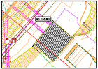
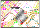
The example shows a small excerpt from a topographical plan as a basis for planning; the initial scale is 1: 250 because of the high information density. It shows a pumping station, the broken edges of the terrain, embankments and roadsides, contour lines and some important pipes. The recorded points with height information, which form the basis of the digital terrain model, were also displayed.

When reducing to a scale of 1: 500 (scaling factor 0.5), the additional height information falls below the legibility limit and is omitted. Only two important and consequently highlighted points are now linked to additional information. The representation can therefore only be used as an overview, because exact height information is now missing.

When enlarged to 1: 100 (scaling factor 2.5), the additional information and the subordinate auxiliary lines are very dominant in comparison with the important terrain break edges, which appear somewhat repressed as a result.

Scale 1: 500 (linear)
Scale 1: 100 (linear)
Scale 1: 500 (non-linear)
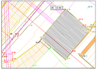
Scale 1: 100 (non-linear)

Improvements through non-linear scaling

A better representation of the additional information within the scope of the possible scaling width brings a scaling with the square root of the scaling factor, so that their area requirement corresponds linearly with the scaling factor of the floor plan geometry. Coupled with an automatic positioning of the text layers according to the resulting free areas, a loss of information can thus be avoided, but not a deteriorated display quality in the border area of the scaling.

The reduction to the scale 1: 500 (scaling factor 0.5 / 0.7) is still possible without any loss of information, but brings the automatic text positioning to the limits of its possibilities. The plan quality is poor but still usable if only a screen view or a temporary work plan in a handy format is required for design purposes.

The enlargement to the scale 1: 100 (scaling factor 2.5 / 1.6) is usable and therefore does not require any rework. Although the auxiliary lines come to the fore a bit more clearly, the additional information remains so reserved that the representation of the important terrain contours is not suppressed.

literature

Stephen Marschner, Richard Lobb: An Evaluation of Reconstruction Filters for Volume Rendering. In: Proceedings of the conference on Visualization '94, pp. 100-107. IEEE Computer Society Press, Los Alamitos 1994, ISBN 0-7803-2521-4 (The article deals with the reconstruction of 3D voxel data , but is also applicable to two-dimensional raster graphics.)
Peter Shirley et al. a .: Fundamentals of Computer Graphics . AK Peters, Wellesley 2005, ISBN 1-56881-269-8 , pp. 99-104
Ken Turkowski, Steve Gabriel: Filters for Common Resampling Tasks. In: Andrew Glassner: Graphics Gems I . Academic Press, Boston 1990, ISBN 0-12-286165-5 , pp. 147-165, worldserver.com (PDF; 160 kB)

Individual evidence

↑ James Foley et al. a .: Computer Graphics: Principles and Practice, p. 515. Addison-Wesley, Reading 1996, ISBN 0-201-84840-6
↑ See for example Video-to-Video Dynamic Super-Resolution for Grayscale and Color Sequences. In: EURASIP Journal on Applied Signal Processing , 2006, Article ID 61859, doi: 10.1155 / ASP / 2006/61859 , people.duke.edu (PDF; 3.2 MB)
↑ See for example Daniel Glasner et al. a .: Super-Resolution From a Single Image . ICCV (IEEE International Conference on Computer Vision) 2009
↑ See for example Johannes Kopf, Dani Lischinski: Depixelizing Pixel Art. ACM Transactions on Graphics 30, 4 (July 2011): 99: 1–99: 8, ISSN 0734-2071 ( online )
↑ hq3x Magnification Filter ( Memento from February 8, 2008 in the Internet Archive )

[1] James Foley et al. a .: Computer Graphics: Principles and Practice, p. 515. Addison-Wesley, Reading 1996, ISBN 0-201-84840-6

[2] See for example Video-to-Video Dynamic Super-Resolution for Grayscale and Color Sequences. In: EURASIP Journal on Applied Signal Processing , 2006, Article ID 61859, doi: 10.1155 / ASP / 2006/61859 , people.duke.edu (PDF; 3.2 MB)

[3] See for example Daniel Glasner et al. a .: Super-Resolution From a Single Image . ICCV (IEEE International Conference on Computer Vision) 2009

[4] See for example Johannes Kopf, Dani Lischinski: Depixelizing Pixel Art. ACM Transactions on Graphics 30, 4 (July 2011): 99: 1–99: 8, ISSN 0734-2071 ( online )

[5] q3x Magnification Filter ( Memento from February 8, 2008 in the Internet Archive )