Superposition (mathematics)

Under superposition property or superposition principle (of lat. Super and positio ; . Dt overlay ) is understood in the mathematics a fundamental property of homogeneous linear equations , after all linear combinations of solutions of the equation results in additional solutions to the equation. With the help of the superposition principle, the solutions of inhomogeneous linear equations can be represented as the sum of the solutions of the corresponding homogeneous equation and a particulate solution. The superposition principle is often used for linear equations that are difficult to solve, such as linear differential equations , in that the initial problem is reduced to easier-to-solve sub-problems. It has a wide range of applications, particularly in physics .

Basics

The following remarks apply generally to vectors (for example numbers , number tuples or functions ) from a vector space over any field (for example real or complex numbers ).

Linear equations

Solutions of a homogeneous and an inhomogeneous real linear equation with unknowns and ${\displaystyle x_{1}}$ ${\displaystyle x_{2}}$

A determining equation in the unknown is called linear when it is in the form ${\displaystyle x}$

${\displaystyle T(x)=b}$

can be brought, where a linear mapping and the right side is independent of . A mapping is called linear if for constants and ${\displaystyle T}$ ${\displaystyle b}$ ${\displaystyle x}$ ${\displaystyle T}$ ${\displaystyle \lambda }$ ${\displaystyle \mu }$

${\displaystyle T\left(\lambda x+\mu y\right)=\lambda T\left(x\right)+\mu T\left(y\right)}$

applies. A linear equation is called homogeneous if the right-hand side is equal to zero , i.e. if it has the shape

${\displaystyle T(x)=0}$

otherwise the equation is called inhomogeneous. Homogeneous linear equations have at least the trivial solution . ${\displaystyle x=0}$

Examples

The scalar linear equation

${\displaystyle 3\cdot x_{1}+4\cdot x_{2}=0}$

with the unknown is homogeneous and is particularly satisfied by the trivial solution while the equation ${\displaystyle x=(x_{1},x_{2})}$ ${\displaystyle x=(0,0)}$

${\displaystyle 3\cdot x_{1}+4\cdot x_{2}=12}$

is inhomogeneous and is not fulfilled by the trivial solution.

Superposition property

Superposition property using the example of the homogeneous linear equation . The equation is solved by and as well as all linear combinations of these solutions. ${\displaystyle 2\cdot x_{1}-3\cdot x_{2}=0}$ ${\displaystyle (3,2)}$ ${\displaystyle (6,4)}$

If and are two solutions of a homogeneous linear equation, then this equation also solves all linear combinations of the two solutions, da ${\displaystyle {\hat {x}}}$ ${\displaystyle {\bar {x}}}$ ${\displaystyle c{\hat {x}}+d{\bar {x}}}$

${\displaystyle T(c{\hat {x}}+d{\bar {x}})=T(c{\hat {x}})+T(d{\bar {x}})=cT({\hat {x}})+dT({\bar {x}})=0+0=0}$.

In general, this statement also applies to all linear combinations of several solutions to form a new solution.

example

The homogeneous linear equation

${\displaystyle 2\cdot x_{1}-3\cdot x_{2}=0}$

is for example through the two solutions

${\displaystyle ({\hat {x}}_{1}=3,{\hat {x}}_{2}=2)}$ and ${\displaystyle ({\bar {x}}_{1}=6,{\bar {x}}_{2}=4)}$

Fulfills. So are too

${\displaystyle ({\hat {x}}_{1}+{\bar {x}}_{1},{\hat {x}}_{2}+{\bar {x}}_{2})=(9,6)}$

and

${\displaystyle (4{\hat {x}}_{1}+3{\bar {x}}_{1},4{\hat {x}}_{2}+3{\bar {x}}_{2})=(30,20)}$

Solutions to the equation.

Particulate solution

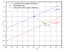
Superposition principle in the linear equation : solution of the homogeneous equation (blue), particle solution (green) and solution of the inhomogeneous equation (red) ${\displaystyle x_{1}-2x_{2}=10}$

In contrast to a homogeneous linear equation, which always has at least zero as a solution, an inhomogeneous equation does not always have to be solvable, that is, its solution set can be empty . If an inhomogeneous equation is solvable, its solutions can be represented as the sum of the solutions of the associated homogeneous equation and a particular solution, i.e. any freely selectable solution of the inhomogeneous equation: Let be a concrete solution of an inhomogeneous linear equation and be the general solution of the associated homogeneous problem , then the general solution of the inhomogeneous equation is da ${\displaystyle {\bar {x}}}$ ${\displaystyle y}$ ${\displaystyle y+{\bar {x}}}$

${\displaystyle T(y+{\bar {x}})=T(y)+T({\bar {x}})=0+b=b}$

applies. This superposition principle is often used to solve inhomogeneous linear equations, since solving the homogeneous linear equation and finding a particular solution is often easier than solving the original problem.

example

A concrete solution to the inhomogeneous equation

${\displaystyle x_{1}-2x_{2}=10}$

is

${\displaystyle {\bar {x}}_{1}=4,{\bar {x}}_{2}=-3}$.

Are now the solutions of the corresponding homogeneous equation ${\displaystyle y=(y_{1},y_{2})}$

${\displaystyle y_{1}-2y_{2}=0}$,

so all with , then the inhomogeneous equation is generally solved by ${\displaystyle y}$ ${\displaystyle y_{1}=2y_{2}}$

${\displaystyle x=y+{\bar {x}}=(y_{1}+{\bar {x}}_{1},y_{2}+{\bar {x}}_{2})=(2y_{2}+4,y_{2}-3)=(2t+4,t-3)}$    with    . ${\displaystyle t\in \mathbb {R} }$

Overlay of solutions

An important application of the superposition principle is the superposition of partial solutions of a linear equation to form an overall solution. If the right-hand side of an inhomogeneous linear equation can be represented as a sum , then the following applies ${\displaystyle b}$ ${\displaystyle b_{1}+b_{2}}$

${\displaystyle T(x)=b_{1}+b_{2}}$,

and are and in each case the solutions to the individual problems ${\displaystyle x_{1}}$ ${\displaystyle x_{2}}$

${\displaystyle T(x_{1})=b_{1}}$   or   , ${\displaystyle T(x_{2})=b_{2}}$

then the overall solution to the initial problem is the sum of the two individual solutions, that is

${\displaystyle x=x_{1}+x_{2}}$.

Such a procedure is particularly advantageous when the individual problems are easier to solve than the initial problem. If the corresponding sums converge, the construction can also be generalized to the superposition of an infinite number of individual solutions. Joseph Fourier used such series to solve the heat conduction equation and thus founded Fourier analysis .

Application examples

Linear Diophantine equations

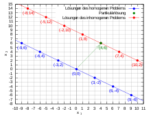
Superposition principle in the linear Diophantine equation : solutions of the homogeneous equation (blue), particle solution (green) and solutions of the inhomogeneous equation (red) ${\displaystyle 2x_{1}+3x_{2}=26}$

→ Main article : Linear Diophantine equation

In linear Diophantine equations , the unknown is an integer vector for the ${\displaystyle x}$

${\displaystyle a_{1}x_{1}+a_{2}x_{2}+\;\cdots \;+a_{n}x_{n}=b}$

should apply, where and are integer coefficients. The solutions of linear Diophantine equations can then be given by combining the solution of the homogeneous equation with a particulate solution that can be found with the extended Euclidean algorithm . ${\displaystyle a_{1},\ldots ,a_{n}}$ ${\displaystyle b}$

example

They are the integer solutions of the linear Diophantine equation ${\displaystyle x=(x_{1},x_{2})}$

${\displaystyle 2x_{1}+3x_{2}=26}$

searched. The solutions of the corresponding homogeneous equation

${\displaystyle 2y_{1}+3y_{2}=0}$

result as

${\displaystyle y=(y_{1},y_{2})=(3t,-2t)}$    with    . ${\displaystyle t\in \mathbb {Z} }$

A particular solution to the inhomogeneous equation is here

${\displaystyle {\bar {x}}=(4,6)}$

whereby the totality of the solutions of the inhomogeneous equation is as

${\displaystyle x=y+{\bar {x}}=(3t,-2t)+(4,6)=(3t+4,-2t+6)}$    With    ${\displaystyle t\in \mathbb {Z} }$

results.

Linear difference equations

Superposition principle in the linear difference equation : solution of the homogeneous equation for the starting value (blue), particle solution for (green) and solution of the inhomogeneous equation for (red) ${\displaystyle x_{n}-2x_{n-1}=3}$ ${\displaystyle x_{0}=1}$ ${\displaystyle x_{0}=0}$ ${\displaystyle x_{0}=1}$

→ Main article : Linear difference equation

In the case of linear difference equations , the unknown is a sequence for which ${\displaystyle (x_{n})_{n}}$

${\displaystyle a_{0}(n)x_{n}+a_{1}(n)x_{n-1}+\;\cdots \;+a_{k}(n)x_{n-k}=b(n)}$    For    ${\displaystyle n\in \mathbb {N} ,n\geq k}$

should apply, where and are coefficients. The solution of a difference equation depends on the starting values . Homogeneous linear difference equations with constant coefficients can be solved, for example, with the aid of the associated characteristic equation . ${\displaystyle a_{0}(n),\ldots ,a_{k}(n)}$ ${\displaystyle b(n)}$ ${\displaystyle x_{0},\ldots ,x_{k-1}}$

example

The first order linear difference equation with constant coefficients

${\displaystyle x_{n}-2x_{n-1}=3}$

results for the start value the result . In order to find the explicit representation of the solution depending on the starting value, one considers the associated homogeneous difference equation ${\displaystyle x_{0}=c}$ ${\displaystyle (2c+3,4c+9,8c+21,16c+45,\ldots )}$

${\displaystyle y_{n}-2y_{n-1}=0}$,

whose solution for the starting value is the result , that is ${\displaystyle y_{0}=c}$ ${\displaystyle (2c,4c,8c,16c,\ldots )}$

${\displaystyle y_{n}=c2^{n}}$

is. A particular solution of the inhomogeneous equation results from the choice of the starting value , which then results in the ${\displaystyle {\bar {x}}_{0}=0}$ ${\displaystyle (3,9,21,45,\dots )}$

${\displaystyle {\bar {x}}_{n}=3(2^{n}-1)}$

applies. Thus the explicit solution of the inhomogeneous problem arises

${\displaystyle x_{n}=y_{n}+{\bar {x}}_{n}=c2^{n}+3(2^{n}-1)=(c+3)2^{n}-3}$.

Linear ordinary differential equations

Superposition principle in the linear ordinary differential equation : solutions of the homogeneous equation (blue), particle solution (green) and solutions of the inhomogeneous equation (red) for varying initial conditions ${\displaystyle f'(x)+xf(x)=(1+x)e^{x}}$

→ Main article : Linear ordinary differential equation

In linear ordinary differential equations , the unknown is a function for which ${\displaystyle f}$

${\displaystyle a_{n}(x)f^{(n)}(x)+\cdots +a_{1}(x)f'(x)+a_{0}(x)f(x)=g(x)}$

shall apply, where are coefficient functions and another function is as right side. The solution of a homogeneous linear differential equation can be given via the associated fundamental system, a particular solution can be found, for example, by varying the constants . ${\displaystyle a_{0},\ldots ,a_{n}}$ ${\displaystyle g}$

example

We are looking for the solution of the inhomogeneous ordinary differential equation of the first order

${\displaystyle f'(x)+xf(x)=(1+x)e^{x}}$

The general solution of the corresponding homogeneous equation

${\displaystyle h'(x)+xh(x)=0}$

is given by

${\displaystyle h(x)=e^{-\int x\;dx}=ke^{-x^{2}/2}}$

with the constant of integration . In order to determine a particular solution, one uses the approach of the homogeneous problem ${\displaystyle k\in \mathbb {R} }$ ${\displaystyle {\bar {f}}}$

${\displaystyle {\bar {f}}(x)=c(x)e^{-x^{2}/2}}$

and tries to find the constant that now depends on. Using the product rule one obtains for the derivation of ${\displaystyle c(x)}$ ${\displaystyle x}$ ${\displaystyle {\bar {f}}}$

${\displaystyle {\bar {f}}'(x)=c'(x)e^{-x^{2}/2}-c(x)xe^{-x^{2}/2}}$

and by substituting in the original equation

${\displaystyle {\bar {f}}'(x)+x{\bar {f}}(x)=c'(x)e^{-x^{2}/2}-c(x)xe^{-x^{2}/2}+c(x)xe^{-x^{2}/2}=c'(x)e^{-x^{2}/2}=(1+x)e^{x}}$

and thus through integration

${\displaystyle c(x)=e^{x+x^{2}/2}}$,

where one can set the constant of integration to zero, since one is only interested in one special solution. Overall, the solution of the inhomogeneous problem is obtained as

${\displaystyle f(x)=h(x)+{\bar {f}}(x)=ke^{-x^{2}/2}+e^{x+x^{2}/2}e^{-x^{2}/2}=ke^{-x^{2}/2}+e^{x}}$.

The solution is then uniquely determined by choosing an initial condition , for example . ${\displaystyle f(0)=k+1}$

Linear partial differential equations

Solution of the homogeneous heat conduction equation with as initial condition ${\displaystyle h_{t}-h_{xx}=0}$ ${\displaystyle 2\sin(\pi x)}$

Particulate solution of the inhomogeneous heat conduction equation with zero initial condition ${\displaystyle f_{t}-f_{xx}=\pi ^{2}\sin(\pi x)}$

Solution of the inhomogeneous heat conduction equation with as initial condition ${\displaystyle f_{t}-f_{xx}=\pi ^{2}\sin(\pi x)}$ ${\displaystyle 2\sin(\pi x)}$

In the case of linear partial differential equations , the unknown is a function of several variables for which ${\displaystyle f}$

${\displaystyle \sum _{\alpha _{1}=0}^{n}\cdots \sum _{\alpha _{m}=0}^{n}a_{\alpha }(x){\frac {\partial ^{|\alpha |}f(x)}{\partial x_{1}^{\alpha _{1}}\cdots \partial x_{m}^{\alpha _{m}}}}=g(x)}$

shall apply, where , and and are coefficient functions. Homogeneous as well as inhomogeneous linear partial differential equations can be solved, for example, using fundamental solutions or the separation approach. ${\displaystyle x=(x_{1},\ldots ,x_{m})}$ ${\displaystyle \alpha =(\alpha _{1},\ldots ,\alpha _{m})}$ ${\displaystyle a_{\alpha }(x)}$ ${\displaystyle g(x)}$

example

The following heat conduction equation is given as an initial boundary value problem

${\displaystyle f_{t}-f_{xx}=\pi ^{2}\sin(\pi x)}$

with the Dirichlet boundary conditions and the initial condition . The solution of the corresponding homogeneous equation ${\displaystyle f(0,t)=f(1,t)=0}$ ${\displaystyle f(x,0)=2\sin(\pi x)}$

${\displaystyle h_{t}-h_{xx}=0}$

with the same initial and boundary conditions one obtains with the help of the separation approach

${\displaystyle h(x,t)=F(x)G(t)}$

with which applies

${\displaystyle h_{t}-h_{xx}=F(x)G'(t)-F''(x)G(t)=0}$

and thus

${\displaystyle {\frac {F(x)}{F''(x)}}={\frac {G(t)}{G'(t)}}}$.

Since the left side of the equation depends only on and the right side only on, both sides must be equal to a constant . So must for and the ordinary differential equations ${\displaystyle x}$ ${\displaystyle t}$ ${\displaystyle k}$ ${\displaystyle F}$ ${\displaystyle G}$

${\displaystyle F''(x)-kF(x)=0}$     and     ${\displaystyle G'(t)-kG(t)=0}$

what is the solution for the given initial conditions ${\displaystyle k=-\pi ^{2}}$

${\displaystyle h(x,t)=2\sin(\pi x)e^{-\pi ^{2}t}}$

results. With the same approach one obtains the particle solution of the inhomogeneous equation with zero initial condition as ${\displaystyle f(x,0)=0}$

${\displaystyle {\bar {f}}(x,t)=\sin(\pi x)(1-e^{-\pi ^{2}t})}$,

which brings the overall solution through

${\displaystyle f(x,t)=h(x,t)+{\bar {f}}(x,t)=2\sin(\pi x)e^{-\pi ^{2}t}+\sin(\pi x)(1-e^{-\pi ^{2}t})=\sin(\pi x)(e^{-\pi ^{2}t}+1)}$

given is.

Applications

→ Main article : Superposition (physics)

The superposition principle has diverse applications, especially in physics , for example in the superposition of forces , the interference of waves , the superposition of quantum mechanical states , heating processes in thermodynamics or network analysis in electrical engineering .

literature

• Hans Wilhelm Alt : Linear Functional Analysis: An Application-Oriented Introduction . 5th edition. Springer-Verlag, 2008, ISBN 3-540-34186-2 .
• Bernd Aulbach : Ordinary differential equations . 2nd Edition. Spectrum Academic Publishing House, 2004, ISBN 3-8274-1492-X .
• Albrecht Beutelspacher : Linear Algebra. An introduction to the science of vectors, maps, and matrices . 7th edition. Vieweg, 2009, ISBN 3-528-66508-4 .
• Peter Bundschuh : Introduction to Number Theory . 6th edition. Springer-Verlag, 2010, ISBN 3-540-76490-9 .
• Gerd Fischer : Linear Algebra: An Introduction for New Students . 17th edition. Vieweg Verlag, 2009, ISBN 3-8348-0996-9 .
• Jürgen Jost : Partial differential equations: Elliptical (and parabolic) equations . 1st edition. Springer-Verlag, 2009, ISBN 3-540-64222-6 .

Web links

Commons : Superposition principle  - collection of images, videos and audio files

• Eric W. Weisstein : Superposition Principle . In: MathWorld (English).