Point operator (image processing)

As a point operators refers to a broad class of image processing operations in the digital image processing , which - compared to local and global operators - are characterized in that in all methods of this class, a new color or gray value of a pixel depending solely on his own previous color or Gray value and its own previous position in the image is calculated without worrying about its neighborhood and / or the context of the pixel.

classification

The generic term point operators includes various frequently used methods of digital image processing such as tonal value correction, contrast enhancement , brightness correction, etc., as well as visualization , and the field of application of point operators in a typical image processing system is correspondingly broad :

scene

→

Image acquisition

→

Preprocessing

→

segmentation

→

Feature extraction

→

Classification

→

Image understanding
visualization

They usually represent the first step in preprocessing in order to increase the image contrast or to compensate for exposure errors during image acquisition. The segmentation of an image is often implemented using a global threshold value method. Following the segmentation, the objects found are often classified , i.e. H. "sorted" into individual classes. When visualizing the results of a segmentation or a classification for humans, the methods of pseudo-coloration or false color display are common.

In addition to the point operators, which transform each pixel of an image individually, there are two further classes of image processing operations in digital image processing with the local operators and the global operators . Local operators always calculate a new color or gray value of a pixel on the basis of a neighborhood or a locally limited region around the pixel. As examples are ranking operators or morphological operators called. Global operators always consider the entire image for the transformation of each pixel, which is the case, for example, with the Fourier transformation .

Most point operators belong to the class of low-level operators . All primitive preprocessing operations, such as noise reduction or contrast enhancement, are combined in this class. A low-level operator means that both the input and the output are an image. In contrast to this are the mid-level operators , which compute a segmentation of an image and extract features of the segments, and the high-level operators , which analyze the interaction of the recognized objects in the image and try to understand the image .

general definition

A point operator T assigns a result image f * to an input image f by transforming the gray values of the individual pixels . The gray value f (x, y) of a pixel (x, y) is only modified depending on the gray value itself and possibly on the position of the pixel in the image:

Transformation of the gray value in the pixel (x, y)

{\ displaystyle f ^ {*} (x, y) = T_ {xy} (f (x, y)) \,}

If the transformation depends on the position of the pixel in the image, it is called inhomogeneous . The indices x and y of T are intended to illustrate this dependency. In the majority of cases, however, homogeneous transformations are used that do not have this dependency. The indices are then superfluous:

{\ displaystyle f ^ {*} (x, y) = T (f (x, y)) \,}

No general statement can be made about the reversibility of such transformations. Some of the procedures presented below, such as B. the negative transformation , are reversible without restrictions. Some other procedures, such as B. the histogram spreading are reversible as long as a continuous gray scale is available. However, if the discrete gray values common in practice are used (see section Application ), rounding errors occur and the transformations are no longer reversible from a strictly mathematical point of view. Most of the time, the rounding errors only have a very slight effect and since the human eye cannot normally perceive the fine difference between two neighboring gray values, the reverse of the transformation subjectively results in the original image. Finally, there are some methods such as B. the histogram limitation , which cannot be reversed, since information is irretrievably lost during use.

A point operator can also be understood as an operator on a neighborhood of size 1 × 1, i.e. a single pixel, and is therefore the simplest form of a neighborhood operator .

application

In practice, the input image of an operation is in most cases a gray value image with a discrete definition range . The value “0” stands for “black”, the value “G” for “white”. G therefore represents the largest possible gray value and is calculated for an image with a color depth of n bits according to the formula: ${\ displaystyle \ lbrace 0, \ ldots, G \ rbrace}$

{\ displaystyle G = 2 ^ {n} -1 \,}

For n = 8 bits, n = 12 bits or n = 16 bits, the three most common gray- scale image formats, G is 255, 4095 and 65535, respectively.

The alternative to a discrete gray scale is a continuous scale. In such an image there is theoretically an infinite number of gray values, which are represented by floating point numbers , usually in the range of values . The term “in the discrete” means that the image is based on a discrete gray scale , while “in the continuous” denotes a continuous scale. ${\ displaystyle \ lbrack 0.1 \ rbrack}$

When applying a homogeneous point operator to an image with a discrete scale, in practice the transformation is often not calculated individually for each pixel. It is sufficient to transform every possible gray value once and save it in a so-called lookup table . The transformation result for each pixel then only needs to be looked up in the table.

Example: An image with a size of 640 × 480 consists of 307,200 pixels. Instead of transforming over 300,000 gray values, with a color depth of, for example, 12 bits, 4096 transformations for all values in the lookup table are sufficient. In addition, there are 307,200 read accesses to the table. With simpler procedures, such as B. the negative transformation , in which only a simple subtraction is carried out, the transformation of a pixel requires less computing time than looking up the table. The use of lookup tables is therefore only worthwhile for more computationally intensive transformations such as histogram spreading .

Since the use of a lookup table is in principle always possible with homogeneous point operators, the transformation T of the gray value f (x, y) of a pixel (x, y) to f * (x, y) defined in the previous section can be more general than the transformation of a Gray value g can be formulated according to g * :

{\ displaystyle g ^ {*} = T (g) \,}

{\ displaystyle {\ text {with}}}

{\ displaystyle T: \ lbrace 0, \ ldots, G \ rbrace \ rightarrow \ lbrace 0, \ ldots, G \ rbrace \ quad {\ text {in the discrete}}}

${\ displaystyle T: \ lbrack 0.1 \ rbrack \ rightarrow \ lbrack 0.1 \ rbrack \ quad {\ text {in continuous}}}$

Histogram with transformation characteristic

The homogeneous mapping of the gray values g of the input image onto the gray values g * in the result image can be described by what is known as a transformation characteristic curve, which is given in discrete form by the lookup table. It is generally not linear, but monotonous over its domain of definition , the gray scale, which at the same time represents its range of values. In the field of digital image processing , the transformation characteristic is called a gradation curve .

The statistical frequencies of the individual gray values in the input image and in the result image can be displayed graphically with the aid of histograms . They enable statements to be made about the gray values occurring, the range of contrast and the brightness of an image and the quality of a possible image segmentation when using a threshold value method.

The mapping behavior of a point operator can be clearly shown using a gray value histogram of the input image, which is superimposed with the transformation characteristic curve used. This form of representation has the advantage that it is relatively easy to read which gray value of the input image is mapped to which gray value in the result image (see example on the left).

Almost all of the methods presented below can in principle also be applied to color images. One possibility is to calculate a common gray value image from the individual color channels of an image and to transform this with the desired point operator. In this case, however, the result is a gray-scale image itself. It gets a little more complicated when the resulting image is again to be a color image. Because a transformation of each individual color channel, for example the red, green and blue channel when using the RGB color space , leads to unsightly to incorrect results. This can be remedied by converting the RGB image into the YCbCr color model . The Y-channel, which shows the brightness, can now be transformed like a gray value image. The image then has to be recalculated back into the RGB color space.

Standard homogeneous transformations

Comparison of the transformation characteristics of power, logarithm, exponential and negative transformations

In the following, some homogeneous point operators will be presented which are widely used in digital image processing, some of which are also used in digital image processing.

Most homogeneous transformations can be divided into two classes: The first class includes the methods whose transformation characteristics always look the same, regardless of which image they are applied to. These include the negative transformation , the power transformation , the logarithmic transformation and the exponential transformation (for a comparison see the adjacent figure). The second class is comprised of the methods whose transformation characteristics are calculated on the basis of the gray value histogram of the input image, i.e. the histogram shift , the histogram spreading , the histogram limitation and the histogram equalization . Only the threshold value method and the pseudocoloring cannot be included in this classification .

Without loss of generality, it is assumed below for all images that they are gray-scale images with a discrete range of values . All the methods presented can also be applied to floating point gray value images. In this case, the rounding is omitted and the normalization factors may have to be adjusted. ${\ displaystyle \ lbrace 0, \ ldots, G \ rbrace}$

Negative transformation

The inversion of the gray values of a gray value image is called negative transformation . Since the human visual system perceives fine differences between gray values in different brightness ranges with different degrees of effectiveness, a negative transformation can lead to a better perception of fine structures. The resulting image is a negative , as is known from analog photography . It can be easily calculated by doing a simple subtraction for each pixel:

{\ displaystyle T _ {\ mathrm {neg}} (g) = Gg. \,}

In contrast to most others, this transformation can be reversed both in the continuous and in the discrete without restriction by repeated application:

{\ displaystyle T _ {\ mathrm {neg}} (T _ {\ mathrm {neg}} (g)) = G- (Gg) = G-G + g = g. \,}

Example image: microcalcification deposits in a female breast ( mammography image)
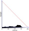
Histogram with transformation characteristic
Image after negative transformation
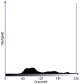
histogram

Power transformation

The power transformation (also called gamma correction ) is a monotonic transformation based on a power function . With this method, the brightness of an image can be changed by carrying out a non-linear spreading for some of the gray values, while the other part is compressed non-linearly.

The parameter specifies the exact behavior of the transformation. If selected, the transformation maps a small number of gray values at the lower end of the scale to a larger value range (the range is spread), while the remaining gray values are projected onto a correspondingly smaller area (this area is compressed). As a result, the picture is brightened. This behavior is more pronounced the smaller is. If you choose, the transformation behaves in exactly the opposite way. A large number of gray values at the lower end of the scale is then compressed and a correspondingly smaller number is expanded at the upper end of the scale. As a result, the larger the image, the more dark it is. The special case is the identity function, i. H. the image is not changed by the transformation. The transformation characteristics for various parameters are shown in the figure above . ${\ displaystyle \ gamma}$ ${\ displaystyle \ gamma <1}$ ${\ displaystyle \ gamma}$ ${\ displaystyle \ gamma> 1}$ ${\ displaystyle \ gamma}$ ${\ displaystyle \ gamma = 1}$ ${\ displaystyle \ gamma}$

Since the transformation must be applied to the value range , the gray values g are first normalized to this by means of division by G. After raising the power to the exponent , the result is normalized back to the desired range by multiplying by G and rounding : ${\ displaystyle \ lbrack 0.1 \ rbrack}$ ${\ displaystyle \ gamma}$ ${\ displaystyle \ lbrace 0, \ ldots, G \ rbrace}$

{\ displaystyle T _ {\ text {power}} (g) = \ left \ lbrack G \ cdot \ left ({\ frac {g} {G}} \ right) ^ {\ gamma} \ right \ rbrack}

The inversion of the power transformation is possible in the continuous without restriction by applying it again with the reciprocal value of the parameter . In the discrete, however, it can only be approximately calculated due to the rounding errors: ${\ displaystyle \ gamma}$

{\ displaystyle T _ {\ text {power}} ^ {- 1} (g) = \ left \ lbrack G \ cdot \ left ({\ frac {g} {G}} \ right) ^ {\ frac {1} {\ gamma}} \ right \ rbrack}

The power transformation offers the possibility of manipulating gray scale or color characteristics of technical devices (e.g. digital camera or monitor). This is necessary in order to adapt the recording or mapping behavior of gray or color values of the individual devices to one another. In this way, the brightness profile of a monitor can also be adapted to the logarithmic brightness perception of the human visual system.


Histogram with transformation characteristics	Histogram a	Histogram b

Logarithmic transformation

The logarithm transformation is a monotonic transformation based on the logarithm . It maps a small gray value range in the lower area of the scale in the input image onto a larger gray value range in the result image, while the upper gray values of the scale are compressed. This will brighten the image as a whole.

Since the value range of the gray values g must first be mapped onto the range by adding 1 before taking the logarithm . In order to obtain a result in the interval from the logarithm function , it is used as a basis . The multiplication by G and the rounding finally normalize the result back to the desired range : ${\ displaystyle \ log (0) = - \ infty}$ ${\ displaystyle \ lbrace 0, \ ldots, G \ rbrace}$ ${\ displaystyle \ lbrace 1, \ ldots, G + 1 \ rbrace}$ ${\ displaystyle \ lbrack 0.1 \ rbrack}$ ${\ displaystyle G + 1}$ ${\ displaystyle \ lbrace 0, \ ldots, G \ rbrace}$

{\ displaystyle T _ {\ mathrm {log}} (g) = T _ {\ mathrm {exp}} ^ {- 1} (g) = \ left \ lbrack G \ cdot {\ frac {\ log _ {2} ( g + 1)} {\ log _ {2} (G + 1)}} \ right \ rbrack = \ left \ lbrack G \ cdot \ log _ {(G + 1)} (g + 1) \ right \ rbrack }

The associated transformation characteristic is shown in a figure above . The inverse of the logarithmic transformation is possible in the continuous without restriction by using the exponential transformation . In the discrete, however, it can only be approximately calculated due to the rounding errors.

The logarithm transformation is often applied to the power spectrum after a Fourier transformation of an image for the purpose of visualization . In such spectra there are often individual points that have a spectral density that is many powers of ten higher than the others. In such a case, simply normalizing all values to the range would result in these outstanding points being displayed with value G and all remaining points with value 0 (see example below). Due to the logarithmic transformation, the high densities are weakened to such an extent that something can actually be seen in the spectrum after normalization. It should be noted that in this application the maximum occurring density must be used as the basis of the logarithm. In contrast to the above, there is no addition of 1, and if the density of a point should have the value 0, it simply has to be mapped to 0 instead of a logarithm. ${\ displaystyle \ lbrace 0, \ ldots, G \ rbrace}$

Example image

Fourier spectrum of the image with value range [0, 2e + 09] normalized to the range {0, ..., 255}

Fourier spectrum of the image normalized to the range {0, ..., 255} after logarithmic transformation

Exponential transformation

The exponential transformation is a monotonic transformation based on the exponential function . It maps a small gray value range in the upper area of the scale in the input image onto a larger gray value range in the result image, while the lower gray values of the scale are compressed. This darkens the image as a whole.

Division by G normalizes the gray values g to the range of values . The value range of the power function is mapped to the desired range by subtracting 1 : ${\ displaystyle \ lbrack 0.1 \ rbrack}$ ${\ displaystyle \ lbrace 1, \ ldots, G + 1 \ rbrace}$ ${\ displaystyle \ lbrace 0, \ ldots, G \ rbrace}$

{\ displaystyle T _ {\ mathrm {exp}} (g) = T _ {\ mathrm {log}} ^ {- 1} (g) = \ left \ lbrack (G + 1) ^ {\ frac {g} {G }} - 1 \ right \ rbrack}

The associated transformation characteristic is shown in a figure above . The inversion of this transformation is possible in the continuous without restriction by using the logarithmic transformation . In the discrete, however, it can only be approximately calculated due to the rounding errors.

Histogram shift

The histogram displacement is a simple method for controlling the brightness of an image. All gray values g of the image are shifted by a fixed constant c on the gray value scale into the light or dark area:

{\ displaystyle T _ {\ text {trans}} (g) = {\ begin {cases} 0 & {\ text {falls}} g + c <0 \\ g + c & {\ text {falls}} 0 \ leq g + c \ leq G \\ G & {\ text {falls}} g + c> G \ end {cases}}}

The histogram shift cannot be reversed, since gray values are always "pushed out" of the scale. An exception is the case when the shifted gray value area in the image was unused.

Example image: The Erechteum on the Acropolis in Athens
Histogram with transformation characteristic
Image after histogram shift with c = -64
histogram

Histogram expansion and compression

Schematic representation of the histogram spread

The histogram spreading , even Gradation called, is a widely used method for improved contrast in low-contrast grayscale images. In such images, many gray values of the gray scale do not appear at all. The larger the unused areas at the two edges of the scale, the more the distance between the darkest and the lightest gray value can be increased, the further the gray values in the image can be "pulled apart".

A gray value spread is calculated using a piece-wise linear transformation that maps the gray value area used to the entire available area : ${\ displaystyle \ lbrace g _ {\ mathrm {min}}, \ ldots, g _ {\ mathrm {max}} \ rbrace}$ ${\ displaystyle \ lbrace 0, \ ldots, G \ rbrace}$

{\ displaystyle T _ {\ text {stretch}} (g) = \ left \ lbrack G \ cdot {\ frac {g-g _ {\ mathrm {min}}} {g _ {\ mathrm {max}} -g _ {\ mathrm {min}}}} \ right \ rbrack}

The reversal of the histogram spreading, the histogram compression (tonal value reduction) , is possible without restriction in the continuous. In the discrete, however, it can only be approximately calculated due to the rounding errors. It reduces the contrast in the image by “pushing” the gray values in the image closer together. In the discrete, the number of gray values used is reduced since gray values lying next to one another are mapped onto a single gray value. Because of this loss of information, the histogram compression is not reversible in the discrete. It is rarely used in digital image processing.

Example image
Histogram with transformation characteristic
Image after histogram spreading
histogram

Histogram limit

If a differentiated consideration of a specific gray value range is desired in a gray value image, a histogram limitation can be carried out. The gray values below and above this area or “cut off” by mapping them to 0 (black) or G (white). The remaining gray values are then contrast- enhanced using a suitable method, typically histogram spreading: ${\ displaystyle (\ lbrace 0, \ ldots, g _ {\ text {min}} - 1 \ rbrace}$ ${\ displaystyle \ lbrace g _ {\ text {max}} + 1, \ ldots, G \ rbrace)}$ ${\ displaystyle \ lbrace g _ {\ text {min}}, \ ldots, g _ {\ text {max}} \ rbrace}$

{\ displaystyle T _ {\ text {clip}} (g) = {\ begin {cases} 0 & {\ text {falls}} 0 \ leq g <g _ {\ text {min}} \\ T _ {\ text {stretch }} (g) & {\ text {if}} g _ {\ text {min}} \ leq g \ leq g _ {\ text {max}} \\ G & {\ text {if}} g _ {\ text {max }} <g \ leq G \ end {cases}}}

The histogram limitation is obviously associated with a loss of information, since it normally maps many gray values on black or white. Therefore it is not reversible.

Example image: The Erechteum on the Acropolis in Athens
Histogram with transformation characteristic
Image according to histogram limitation and spreading
histogram

Histogram equalization

Schematic representation of the histogram equality

The Histogrammäqualisation (also histogram equalization , Histogrammeinebnung , Histogrammegalisierung or Histogrammequalisierung is called) is an important method to improve contrast in gray scale images, which goes beyond a mere contrast enhancement. A uniform distribution is calculated from the gray value distribution in the histogram so that the entire available value range is optimally used.

This method is used in particular in those cases in which the interesting image areas make up a relatively large part of the image (the corresponding gray values therefore occur more frequently than average) and their gray values are limited to a small area of the gray value scale.

In contrast to a histogram limitation with subsequent histogram spreading , where the contrast is increased in the interesting gray value area, but the information outside the area is completely lost, in histogram equalization frequent gray values are "stretched apart" (the gray value scale is stretched in these areas) and less frequent Gray values “pushed together” (the gray value scale is compressed in these areas).

In practice, however, such a beautiful equal distribution as in the schematic diagram opposite will never be achieved. The histogram of the resulting image will rather contain more or less large gaps (see example below). This is due to the fact that a discrete gray value can only be mapped onto another discrete gray value and cannot be “pulled apart”. If a gray value occurs very frequently, its direct “neighbors” on the gray value scale will no longer appear in the image after the uniform distribution.

The so-called cumulative gray value histogram of the image serves as the basis for determining the transformation characteristic . This is calculated by assigning the sum of all relative frequencies H of the gray values 0 to g to each gray value g : ${\ displaystyle H_ {k}}$

{\ displaystyle H_ {k} (g) = \ sum _ {n = 0} ^ {g} H (n)}

This cumulative gray value histogram represents a sequence of values in the interval . By multiplying each sequence element by G and then rounding it up, the transformation characteristic with value range results : ${\ displaystyle \ lbrack 0.1 \ rbrack}$ ${\ displaystyle \ lbrace 0, \ ldots, G \ rbrace}$

{\ displaystyle T _ {\ text {equal}} (g) = \ left \ lbrack G \ cdot H_ {k} (g) \ right \ rbrack}

The histogram equalization is lossy, since larger areas of the scale with gray values of low frequency are compressed to a few gray values. Therefore it is not reversible.

Example image : Small crater on Mars (shot of the opportunity rover)	(a) Image after histogram equalization	(b) Image after histogram hyperbolization with α = -1/3
Histogram with transformation characteristics	histogram	histogram

Histogram hyperbolization

After a histogram equalization , the gray values in the resulting image are evenly distributed, but this often looks too bright for a human observer. This is because the brightness perception of our visual system is not linear, but logarithmic. Using a histogram hyperbolization instead of an equalization, the gray values are adapted to the subjective human perception:

{\ displaystyle T _ {\ text {hyper}} (g) = \ left \ lbrack G \ cdot H_ {k} (g) ^ {\ frac {1} {\ alpha +1}} \ right \ rbrack}

The transformation characteristic of the uniform distribution is shifted somewhat in the direction of a hyperbolic course. The dark gray values are more likely than the light ones, which means that the image is darkened overall. can assume values from the interval . Values from to are common , for the hyperbolization corresponds to the equality. If the gray value 0 is dispensed with, a logarithmic probability distribution of the gray values can be achieved with. ${\ displaystyle \ alpha}$ ${\ displaystyle \ rbrack -1.0 \ rbrack}$ ${\ displaystyle \ alpha = -2 / 3}$ ${\ displaystyle \ alpha = -1 / 3}$ ${\ displaystyle \ alpha = 0}$ ${\ displaystyle \ alpha \ rightarrow -1}$

Since the histogram hyperbolization is based on the non-reversible histogram equalization and is similarly lossy, it is also not reversible.

Global threshold value procedure

Global threshold value methods are often used in the area of image segmentation . Each pixel of a gray value image is assigned to one of two classes on the basis of its gray value. In this way, for example, the foreground of the image is often separated from the background or a distinction is made between objects of different lightness. The boundary between the two classes is determined by a threshold value t :

{\ displaystyle T _ {\ text {thresh}} (g) = {\ begin {cases} 0 & {\ text {falls}} g <t \\ 1 & {\ text {falls}} g \ geq t \ end {cases }}}

The application of the threshold leads to a binarization of the image, i. H. the resulting image only contains the values 0 and 1. If the color depth of the image is to be retained, the gray values can alternatively be mapped to 0 (black) and the largest possible gray value G (white):

{\ displaystyle T _ {\ text {thresh}} (g) = {\ begin {cases} 0 & {\ text {falls}} g <t \\ G & {\ text {falls}} g \ geq t \ end {cases }}}

However, such a separation can only function optimally if a bimodal histogram is available as in the example below, i.e. if there are two local maxima in the histogram. There are various approaches to choosing an optimal threshold value, the best known among the non-trivial ones is probably the Otsu method .

In addition to the global ones, there are also local threshold value methods . However, these are not point operators, because with them the threshold values are set individually for each region or each pixel on the basis of a small image region or a neighborhood .

Further information on this topic can be found in the article Threshold method .

Example image

Histogram with transformation characteristic

Image after segmentation with threshold value 90

Pseudocoloring

Thermal image of a dog

The Pseudokolorierung is a process for coloring intensity images, such as thermal imaging , to make small differences in brightness within an image more visible. This is done by mapping the definition range of the intensity values (which can be understood as gray values) on a higher-contrast color scale. A vector is assigned to each intensity value g : ${\ displaystyle {\ vec {g ^ {*}}}}$

{\ displaystyle {\ vec {g ^ {*}}} = (r ^ {*}, g ^ {*}, b ^ {*}) ^ {T} = T (g)}

The composition of the vector is determined by the color space used. In this case, the three components r * , g * and b * stand for the red, green and blue color components in the RGB color space . ${\ displaystyle {\ vec {g ^ {*}}}}$

One problem that must be taken into account with this method is the different brightness perception of the human visual system for different colors. For example, humans perceive a yellow area much lighter than a blue area of the same intensity. The selection and sequence of the individual colors for the color scale is therefore not arbitrary. Subjectively “dark colors” such as blue or purple are used at the lower end of the scale, while the “light colors” are used at the upper end of the scale. This can be seen very nicely in the example opposite, where the color scale used is shown to the right of the colored thermal image of a dog. Since the sequence of the individual color values is not trivial, it can often not be described by a simple function. For this reason, a lookup table is usually used with this method, which in this special case is also called a color map .

It is also possible to map the color values of a color image onto another color scale. This so-called false color display works similarly to pseudocoloring, the only difference being that a different vector is assigned to each color component vector : ${\ displaystyle {\ vec {g}}}$ ${\ displaystyle {\ vec {g ^ {*}}}}$

{\ displaystyle {\ vec {g ^ {*}}} = (r ^ {*}, g ^ {*}, b ^ {*}) ^ {T} = T ({\ vec {g}}) = T ((r, g, b) ^ {T})}

Inhomogeneous standard transformations

Inhomogeneous point operators are generally used much less frequently than the homogeneous operators. This is due, on the one hand, to the fact that the use cases are simply not given that often and, on the other hand, to the fact that the implementation of many methods is non-trivial. Two selected simple inhomogeneous transformations are presented below.

Correction of inhomogeneous lighting

In scientific test series, the test set-up of which includes image recordings, for example recordings of cell cultures or microscopic images of cells in liquid, various disruptive effects can occur which sometimes significantly disrupt the further processing of the images. Despite the great effort involved in setting up the experiment and the greatest care, there is always (even if only minimally) uneven lighting of the scene. Another source of interference are small dust particles on a lens or on the glass in front of the CCD sensor . These are only recorded very blurred because the focus of the camera is in a different area and are not directly visible in the image, but they absorb light and reduce the brightness in part of the image. Another problem with devices with digital recording technology, especially when inexpensive CMOS sensors are used, is an uneven sensitivity of the individual photoreceptors .

All of these effects make image analysis difficult, especially the segmentation of objects and the background. This can go so far that the background is darker than the objects in some places and segmentation with a global threshold value becomes completely impossible. If, however, a reference image was taken before or after the experiment, i.e. an image of the unevenly illuminated scene under experimental conditions, but without objects, the above-described interference effects can be eliminated and the resulting image ideally has a white background with homogeneous brightness. It is calculated by dividing the test image f point by point by the reference image and then normalizing it to the desired value range : ${\ displaystyle f ^ {*}}$ ${\ displaystyle f_ {r}}$ ${\ displaystyle \ lbrace 0, \ ldots, G \ rbrace}$

{\ displaystyle f ^ {*} (x, y) = T_ {xy} (f (x, y)) = \ left \ lbrack G \ cdot {\ frac {f (x, y)} {f_ {r} (x, y)}} \ right \ rbrack}

Under certain circumstances, this method can still be used even if no reference image exists for a series of experiments. Because if the recorded objects are small and randomly distributed in the images, there is the possibility of using an average value image from several or all images in the series as a reference image.

Objects against an unevenly lit background

Unevenly lit background

Fixed uneven lighting

Window function

For the calculation of the Fourier transform of an image, this is assumed to be periodic. If, however, there is no possible periodicity , that is to say the left and right or the upper and lower image edges have different brightnesses or structures, a periodic repetition leads to discontinuities at the image edges. These are visible in the spectrum as high spectral densities along the axes (see example below). If further operations in Fourier space are used, for example a convolution with a smoothing operator, these high densities can be considerably disruptive.

The disruptive effect can be avoided by multiplying the image f with a suitable window function w , which assumes values in the interval and drops to 0 from the center to the edge of the image: ${\ displaystyle \ lbrack 0.1 \ rbrack}$

{\ displaystyle f ^ {*} (x, y) = w (x, y) \ cdot f (x, y)}

Using a cosine window as an example (as in the example below) results in the following transformation rule, where X and Y represent the number of pixels in the x and y directions:

{\ displaystyle f ^ {*} (x, y) = \ sin {\ left (\ pi \ cdot {\ frac {x} {X}} \ right)} \ cdot \ sin {\ left (\ pi \ cdot {\ frac {y} {Y}} \ right)} \ cdot f (x, y) \ qquad {\ text {with}} 0 \ leq x <X, 0 \ leq y <Y}

Of course, the windowing of the image also changes the entire spectrum slightly.

Example image
Fourier spectrum of the image (high spectral densities along the axes)
Windowing of the example image
Fourier spectrum of the windowed image

credentials

literature

Thomas Lehmann, Walter Oberschelp, Erich Pelikan, Rudolf Repges: Image processing for medicine: fundamentals, models, methods, applications. Springer-Verlag, Berlin 1997, ISBN 3-540-61458-3
Bernd Jähne : Digital image processing. 6th, revised and expanded edition. Springer-Verlag, Berlin 2005, ISBN 3-540-24999-0
Rafael C. Gonzalez, Richard E. Woods: Digital Image Processing. 2nd edition, Prentice Hall, 2001, ISBN 0-20-118075-8 (English)

Web links

Image processing for medicine by Thomas Lehmann and others as download version (PDF 6.2 MB)
Image processing in practice by Rainer Steinbrecher in the 2nd revised edition as a download version (PDF 6.1 MB) (1st edition: ISBN 3-486-22372-0 )