Welding process monitoring

Through process monitoring the quality of a product should monitored during ongoing production and ensuring that the quality requirements are met. In contrast to this, the condition monitoring of production plants permanently controls the condition of the plant by measuring physical quantities and is convinced of the trouble-free plant functionality.

Process monitoring in industrial production records essential physical measured variables that characterize the production quality or features derived from them during the ongoing process and evaluates the process. The result is a statement about the expected quality of the finished product. In this way, a full test of all manufactured products is sought. Online process monitoring closely couples the quality assessment with the manufacturing process so that there is as little time loss as possible between its completion, the quality statement and a possible reaction of the manufacturing plant to the quality result.

In the online welding process monitoring is the quality assessment of welded joints during or immediately after completion of the welding process. Online welding process monitoring facilities often combine the functions of quality monitoring with those of the condition monitoring of production systems .

Basics and terms of online process monitoring

The quality values ​​of welded joints (quality features ) cannot be measured directly with the help of process monitoring. Instead, conclusions are drawn about the quality by means of correlating quality substitute variables (monitoring features). For this purpose, objects that are to be assessed are compared with a group (a class) of objects that are known to meet the quality requirements. The result of the comparison is an assessment of the similarity of the object with the set of all known objects. The theoretical basis for this is provided by methods of classification , i. H. combining objects into classes and assigning unknown objects to an existing class system ( classification ) using a classifier .

object

Feature vector of the dynamic resistance of a resistance spot welding as a profile plot

Objects are represented in the given context by features of a welding process obtained from measured values. In the case of a single feature, the object is a scalar quantity. If several features are used for the object description, the object can be understood as a feature vector in the multi-dimensional feature space and graphically represented by a point in the Cartesian coordinate system . For feature vectors with dimensions greater than three, the profile display (profile plot) or the display in polar coordinates (polar plot, network diagram ) are suitable (see graphic display of objects and classes ).

Example: A resistance spot is determined by the measurement variables voltage and welding current characterized. The heating of the sheets and thus the size of the weld point that is created reflects the resistance. Since both variables change during the connection formation ( dynamic resistance ), the resistance mean value should be calculated from the effective values ​​of both variables. In this case, this scalar variable represents the object “resistance welding point”. For a closer look, you can increase the resolution of the measurement and use mean measured values ​​of the electrical quantities over a time window (e.g. every 20 ms), from which the quotient is formed. A sequence of measured values ​​results, the components of which can be understood as a feature vector. It can be visualized graphically using a profile display.

Signals and features

The monitoring features are extracted from measurable physical process variables. The process signals and the characteristics derived from them must have a high correlation with the quality if they are to be used for quality assessment. The question of which process signals and characteristics should be used for a special monitoring task cannot be formally answered. Process analyzes can only clarify which signals and derived characteristics show sufficient correlation with product quality.

Requirements for characteristics

In general, features should meet the following requirements:

• they must show clear functional relationships with at least one or more quality features and in this way enable the clearest possible assignment of quality,
• A process change without a quality change must not have a relevant influence on the feature vector,
• the interference level of the process signals must be significantly lower than the signal change due to relevant process disturbances,
• when using several features, the correlation between the features should be as low as possible.

Feature correlation

Correlating features have no additional information for the classification. Correlation between features leads to rotated classes in the feature space. The rotation has an adverse effect on the classification. If the class z. B. is described by sharp, axially parallel borders, this means that the area of ​​validity extends into the corners of the circumscribed rectangle (red areas in the adjacent picture). However, these areas are actually outside the class, because the class is only represented by the objects shown in green. Objects with characteristic values ​​within the red area (blue objects) are mistakenly regarded as belonging to the class. This can be avoided by using class descriptions that take this class rotation into account (e.g. kernel density estimation or fuzzy pattern class description ). A feature pretreatment is also possible, which transforms the features in such a way that correlation is avoided ( principal component analysis , discriminant analysis or independence analysis ).

class

Three natural classes make up a semantic class

Class description through axially parallel class boundaries for correlating features

Example of one-dimensional sharp and fuzzy membership functions over the associated learning objects

Classes are sets of objects with similar characteristic values, e.g. B. all resistance welds with an average resistance value within certain minimum and maximum limits or those that can be assigned to the quality "OK - OK". The similarity can be determined according to content ( semantic ) or formal criteria. In this way, semantic and natural classes can be distinguished. Semantic classes summarize objects that are similar in terms of content (e.g. quality). Natural classes consist of formally similar objects. This distinction is useful for process monitoring. The aim of the monitoring is to establish an extensive correspondence between quality classes (semantic) and the natural classes (formal). In the automated monitoring process, only natural classes can be dealt with, whereby the semantic class “OK - OK” can often only be represented by several natural classes in order to achieve the necessary quality of classification. Then a semantic class is mapped by several natural classes.

Disjoint, nondisjoint, sharp and fuzzy classes

Classes can be disjoint ; H. they are limited by sharp edges. All objects with characteristic values ​​within the sharp limits belong only to this class, all other objects do not. Such classes are rare in the real world. Objects there belong more or less strongly to one class, often they also have more or less pronounced properties and thus characteristic values ​​of other classes. The classes are not disjoint, and the boundaries are fluid. Since no class boundaries can be described, these classes are mapped by distribution functions, which can be understood as membership functions. The membership function assigns a number from the real-valued interval to each object of the feature set , which number indicates the degree of membership of the object to the fuzzy set defined in this way . Instead of the term degree of membership , membership value or sympathy value is also used. ${\displaystyle \mu _{KL}:X\rightarrow [0,1]}$ ${\displaystyle x}$ ${\displaystyle X}$ ${\displaystyle [0,1]}$ ${\displaystyle \mu _{KL}(x)}$ ${\displaystyle KL}$

Graphical representation of objects and classes

Radial plot of multiple objects and classes with five characteristics

Profile plot of multiple objects and classes with five characteristics

Example of a scatter plot for three natural classes with five characteristics

Classes from objects in the higher-dimensional feature space can, like the objects, be graphically represented by radial or profile plots. Colored, multidimensional scatter diagrams are a special form of graphical representation of objects in a class . Two features are visualized in a matrix of 2D representations. Since one side of the matrix diagonal is sufficient for this, the frequency distributions of the objects over a feature can be displayed on the diagonal and the correlation coefficients between the features on the other side.

Object and class equality or similarity

Euclidean distance between two objects in the two-dimensional Euclidean feature space

Comparison of the Euclidean and Mahalanobis distances of two objects to the center of a class

Automatic monitoring by computers can only work with formal equality or similarity. Equality or similarity is expressed by distances in the feature space. If an object (or a class) is within a defined distance to the other, it can be regarded as the same. Since most of the features in online process monitoring are explained on metric scales , the Euclidean distance is often used to determine the similarity. It is the direct distance between two objects in the Euclidean feature space .

If features correlate with one another, the Euclidean distance in the direction of the correlation axis expresses an apparent difference between the objects. If the correlation is to be taken into account in the distance calculation, the Mahalanobis distance can be used to calculate the object similarity. This is explained using the following example. The Euclidean distances of the objects O1 and O2 to the center of gravity of all objects M [0,0] are the same and are each 2. The ellipses in the adjacent figure are the estimates (0.1%… 99.9%) of the Gaussian distribution for the given objects . The two features M1 and M2 lie on the ellipse 1 (0.1%) and 6 (50%), so have very different distances to the center with regard to their variances, while the Euclidean distance of both objects to the center is the same. This difference is represented by the Mahalanobis distance.

Objects in two groups with one object (red) in the first group

Similarity of objects to an individual object (red) according to the Euclidean distance and taking into account the rank in the group. (The size of the blue circles corresponds to the similarity)

In addition to geometric distances, similarity between objects can also be defined by taking into account the internal distribution structure of the objects in the feature space. Example: The picture opposite shows objects that are clearly arranged in two groups in the two-dimensional feature space for a human observer. They each have a similarity to one another, which is supported by their mutual closeness, by their rank within a group. If the similarity of an object to all other objects is determined solely by the distance, some objects in both groups have a greater similarity to this object than objects in their own group. If the rank of the objects within the group is taken into account, the picture is clearly different. For the consideration of the rank for the distance calculation, Zhou et al. a. developed an algorithm ( Ranking on Data Manifolds ).

The choice of distance measure is very important for the assignment of individual objects to a class.

Process monitoring

Process monitoring by evaluating individual objects

Classification procedure

For quality control statistical pattern recognition method based on supervised classification are ( supervised learning , supervised learning ) are used. The classification processes must be manageable in real time in the automated manufacturing process. The entire monitoring process has two phases:

• Learning (training) and validation phase
• Application phase

Training phase

In the training phase, the manufacturing process is monitored over a certain period of time. Values ​​of monitoring features ( feature vectors ) are obtained and stored. The quality of the individual connections is measured and stored together with the feature vectors. The degree of process stability and process capability during this manufacturing period is determined. If the process is mastered and capable , the set of all stored feature vectors (learning objects) forms the basis for the semantic OK class. A classifier is calculated from this using a mathematical description (class description). This process is known as supervised learning. The classifier is saved and is used in the application phase to evaluate unknown feature vectors.

Before each class description from existing sample objects, a definition is made as to which objects belong to the OK class. This assessment is carried out by an expert (teacher). For pragmatic reasons, only one semantic class - the OK class - is formed for process monitoring, because for reasons of cost and effort, technological protection can only be carried out for the OK processes that have occurred. It is impossible to support all conceivable process situations and thus also processes of insufficient quality with sample data.

The OK class can contain objects from different technological process situations. The feature values ​​within the semantic OK class differ in this case to a greater or lesser extent and it can then consist of several natural subgroups, each of which corresponds to a technologically similar state. The structure of formally similar subclasses can be found using clustering methods.

Description procedure for classes

Class description by envelope curves of the dynamic resistance in resistance spot welding in profile representation

Description of classes by class boundaries in the feature space. The class boundaries have been calculated by SVM .

Membership function of a bimodal class in the feature space calculated by fuzzy pattern classification (separation into two subclasses)

Membership function of a bimodal class in the feature space calculated by kernel density estimation

Relearning objects from dynamic resistances in resistance spot welding

Before the class description, there are data sets of feature vectors with class assignment, which are provided by an expert (teacher) after possibly formal separation into natural compact subclasses.

A natural class has a position and dispersion in the feature space, the location of which in the feature space must be described using mathematical means. This is the only way to automatically assign unknown objects. This process is called class description. A wide variety of concepts have been developed for this:

• Description by clear class boundaries (e.g. separation functions or envelopes ),
• Description by means of distribution functions (e.g. by means of kernel density estimation , EM algorithm with Gaussian Mixture Models or fuzzy pattern class description ).

The result of a class description is a classifier as an instance for the class assignment (classification) of unknown objects to one or more defined classes.

Re-learning and class separation

The welding processes are generally time-variant ; H. they change their behavior over a certain period of time due to wear and tear and changes in the technological situation without the quality results necessarily having to change significantly. In order to take this into account, it must be possible to relearn in the subsequent work phase (use of the classifier).

The re-learning can lead to an excessive local expansion of the class, which, depending on the description method, leads to a deterioration in the classification. This can prevent the class from being split into individual compact subclasses. To this end, methods of unsupervised learning , e.g. B. cluster method applied.

The picture on the right shows an example of class formation in resistance spot welding. The features are samples of the dynamic resistance . The classes are made up of sample objects. After further welding, new objects outside of the class appear, which are found to be good after an examination. The objects are added to the class. The class is getting wider. When using the class description using envelope curves , the classification deteriorates. The class is split into two sub- classes by k-means clustering , which are described separately by envelopes and used for classification.

Application phase

In the application or monitoring phase, the feature vectors of the current process are calculated in real time. They are compared with the given IO classes with the help of the classifier. All feature vectors outside this range or below a membership value threshold are assessed as not in order (not OK). In this case, the production control can be intervened. The evaluation results are saved, statistically evaluated and made available for visualization.

Components of a system for welding process monitoring

Scheme of online process monitoring through supervised learning

A monitoring system is a hardware-software system. It has technical means to carry out all sub-tasks including human-machine communication. It is technically integrated into the production workstation, which in the simplest case consists of a welding tool (welding machine, welding gun, welding torch) that is operated by a person. In complex cases, several robots, welding guns, components and welded joints must be monitored at the same time. Apart from the increased complexity, nothing changes in the basic technical concept. The picture on the right shows the basic scheme of such a system.

The hardware consists of components for measured value processing including sensors and measured value transmission, signal processing, data storage, operation and visualization.

Software modules control the measurement of the process variables and the calculation of the characteristics. In the learning or training phase, classifiers are calculated from the feature data of tested learning objects and stored (classification). For this purpose, the test results of the learning objects must be available and archived in order to be able to prove the tested quality of the learning objects at any time. Once valid classifiers are available, the process features are used in the application phase to compare the current feature vectors with the classes (classification). The comparison result is a quality assessment of each individual welded joint. A feedback to the system control can be generated from this. The monitoring results are archived in databases and are available for statistical evaluations. The compressed evaluation results are visualized in real time. This results in indications for process improvement.

Process monitoring through observation and evaluation of process stability

Adaptive visualization according to Müller and Holweg

Online monitoring systems can also be used to assess process stability. Leaving the technologically required process window is signaled in good time and corrective measures can be initiated. In this way, functions of the system condition monitoring are integrated into online monitoring systems in order to avoid malfunctions of the welding process due to system malfunctions such as poor electrode condition , malfunctions in the power or cooling system, changes in the workpiece surfaces and the like. to recognize and to stop early. This procedure is called adaptive process visualization in the VW standard PV 6702 . Measured data are saved and visualized using a special form of profile display. The feature values ​​of each individual weld (object) are plotted sequentially over a running variable, e.g. B. each weld is represented by its characteristic curve over time. From the set of all objects stored from a start value up to the current point in time, frequency distributions are calculated for each characteristic (reference value of the run variable). The current frequency is visualized by a color value. During a running process, the frequency distributions change their shape and position dynamically. This creates a dynamic statistical image of the process. The variance can be seen directly from the coloring. A statistically largely invariant process is characterized by a sharp color band; a strongly varying process will change both its shape and position and the sharpness of its colored contour.

Online process monitoring in the manufacturing process

structure

In order to trace the quality of the welded joint, each individual joint must be identified by a unique signature. It must be clear from it at which welding workstation the component and the special connection was welded and when. Each welding device has its own identification, which is combined with a component and connection number and a time stamp for a unique identification number after the welding has been completed. This signature is archived together with the result of the quality assessment and the actual values ​​of the welding parameters .

For permanent process improvement it is advantageous to have the position on the component, the material quality and surface properties, the material dimensions and the set welding parameters available in the system for each connection.

A monitoring system should be able to generate the welded connection numbers and conveniently archive them together with the information mentioned and make them available via a visual human-machine interface .

Integration of monitoring systems in a manual workstation

Integration of a monitoring system in a manual workstation for resistance spot welding

Integration of a monitoring system in a robot welding cell for resistance spot welding

Depending on the welding process, the workplace consists of a welding machine or welding tongs for resistance welding or a welding power source and a welding torch for arc welding with a clear device identification. It is equipped with sensors for measuring the monitoring parameters. The workpiece is held by a device and manipulated if necessary. An operator guides the workpiece to the welding tool (in resistance welding) or the welding tool to the workpiece (in arc welding). The welding process is triggered by the operator via the welding control.

The sensor signals are fed to a module for feature calculation and process monitoring via measuring lines. These are the only communication channel between the monitoring system and the plant. The start and end of monitoring are signaled by the start of the current flow ( trigger ). An internal counter generates a connection number and counts the number of connections. If a preset number of connections is reached, the end of the component is signaled and a component number is generated. If this simple solution is too insecure, the start and end of the component (trigger) and the respective connection number must be generated by control measures. Data is archived for each component and connection number.

Integration of monitoring systems in complex production

Complex components such as B. a body, are manufactured in complex welding systems that consist of several welding stations with numerous welding robots. Each robot can operate several change pliers during resistance welding .

The workpiece is held and manipulated by devices. Robots guide the welding tool to the workpiece (or the workpiece to the welding tool) with their own identification. The robot controls ensure the correct production process; they may also take over the tasks of the manipulator, gun and welding controls. The controls provide information about the current welding process. Station, robot, gun, torch, component and weld joint number ready. The switch-on and switch-off signals for process monitoring are also triggered by the controller and taken over by the monitoring system.

Visualization of a monitoring system

Play media file

Visualization options with a monitoring system in complex production for resistance spot welding

In addition to the monitoring function, an essential function of online monitoring systems is the provision of information about the entire welding process. This is the only way to permanently improve the process quality. Various concepts for the representation of process information have been developed. Ultimately, they are all based on more or less complex visualizations. The film on the right shows the structural possibilities of such visualization.

Online process monitoring for resistance welding

Monitoring sizes and characteristics

Due to their different physical mechanisms of action, the welding processes each place specific requirements on the selection of the monitoring parameters and features, the process evaluation methods used, the time and the type of process evaluation in the manufacturing process.

Generally accepted quality features in resistance spot welding are the spot diameter d _P (determined by a workshop test) or the lens diameter d _L (measured on a macro cross-section ). These variables cannot be measured directly in the monitoring process either, but characteristics for monitoring must be obtained from measurable physical variables.

Monitoring quantities

The point diameter depends on the time course of electrical heating . This results in potential monitoring variables:

• the welding current,
• the welding voltage,
• the welding power and the dynamic resistance as combined quantities of current and voltage
• the welding current time.

The force acting on the welding point influences the transition resistance and thus the heating process. As the material heats up, its volume increases, which creates a force on the electrode. This force is proportional to the heating. From these considerations it follows that the electrode force and the electrode return stroke (electrode travel) and variables derived from them such as electrode speed and electrode acceleration can also provide information about the formation of the connection.

The formation of the connection is accompanied by a sound emission, so that information about the connection can also be searched for in the sound.

Provides an overview of the monitoring parameters examined in the past.

Monitoring features

Features that correlate with the spot welding quality are generated from the measured process signals .

Characteristics from electrical quantities

AC welding

The phase control, voltage and current curve at mains frequency

Features of cut alternating current

Dynamic resistance when direct current welding of sheet steel

Features that can be obtained from the current in AC welding are the peak or peak value and the rms value . In AC welding, the current is changed by phase control . The duration of the actual current flow per half-wave is referred to as the current flow time in ms or, based on the entire half-wave of at or at, as the current flow angle in ° (degrees). The inductance of the secondary circuit results in a phase shift with a load angle between voltage and current . From this, the calculated effective power to . The size of the power factor is essentially determined by the window opening of the secondary circuit of the welding gun. All of the variables mentioned can be used for monitoring AC welding. ${\displaystyle t_{F}}$ ${\displaystyle 180^{\circ }=10\;\mathrm {ms} }$ ${\displaystyle 50\;\mathrm {Hz} }$ ${\displaystyle 8{,}33\;\mathrm {ms} }$ ${\displaystyle 60\;\mathrm {Hz} }$ ${\displaystyle \delta }$ ${\displaystyle \phi }$ ${\displaystyle P}$ ${\displaystyle P=U\cdot I\cdot \cos \phi }$ ${\displaystyle \cos \phi }$

Dynamic resistance

Play media file

Development of dynamic resistance in resistance spot welding of unalloyed steel

Dynamic resistance and point diameter with increasing energy input

When welding with all types of current, the heating and connection formation and ultimately the size of the nugget depend on the development of the resistance over time during the physical processes taking place at the welding point. The lens formation is clearly reflected in the so-called dynamic resistance . In addition to the material temperature, it also depends on the material and surface properties of the joint partners.

A similar resistance curve for different welds with the same physical properties of the joining partners (material) indicates similar lens formation. When welding unalloyed steel sheets with a bare surface, the total resistance runs through three time periods:

1. In the first section, the resistance drops sharply and is determined by the surface condition of the workpieces and the electrodes. When the sheets are pressed together, it sinks within a short time.
2. The material resistance increases due to the increase in temperature at the contact point, while at the same time the electrodes penetrate the workpiece as the material softens. The current path and with it the resistance fall.
3. In the final phase, the material resistance decreases as a result of the strong electrode penetration into the workpiece.

These processes are superimposed so that the dynamic resistance gets its characteristic course.

Relationship between dynamic resistance and point diameter

The change in the point diameter and the shape and position of the dynamic resistance as a result of the changed energy input are shown in the pictures (2 × 1.5 mm sheet steel H320 with coated surface). The energy was changed by varying the current. If the energy input is too low, the resistance runs flat, the point diameters are smaller than necessary (red). With increased energy, the point diameter grows and exceeds the required specification limit. The dynamic resistance increases and a pronounced relative maximum forms (green). With a further increase in energy, the maximum shifts to an earlier point in time. The drop in resistance after passing through the relative maximum becomes steeper with increasing energy. After the spatter limit is exceeded, the spot size fluctuates due to the loss of material due to spatter. Splashes can be seen as a steep drop in dynamic resistance (magenta).

Features from dynamic resistance

Features from dynamic resistance as mean values ​​over a time window of 20 ms

Characteristic formation from the dynamic resistance

For process monitoring with the help of dynamic resistance, features must be found that represent an image of form and position. In the simplest case, sampling values ​​r _s (t) averaged over a time window can be used. The advantage of this procedure is that any curve shape can be simulated without any problems. The number of features then depends on the welding time, which has a disadvantageous effect on practical handling. In addition, these features correlate to a high degree in the area of ​​increasing or decreasing course. In this case, it makes sense to use additional  axis transformations for the pretreatment of characteristics.

Features that are independent of the welding time and largely free of correlation are more favorable than a direct mapping of the dynamic resistance using support values. For the dynamic resistance with a pronounced relative resistance maximum, as it is formed when welding unalloyed steel sheets, the following geometric quantities are available:

• the height of the relative maximum: R _max
• the time of minimum resistance R _min after the application of force t _min
• the time at which R _max t _{max is reached}
• the slope R from the minimum R _min to the reaching of R _max   dR ₁
• the slope from R _max   to the end of welding: dR ₂

This also enables the shape and position of the course to be clearly reproduced.

Features from mechanical quantities

As a result of the ohmic heating of the joining partners at the welding point, the material expands locally. There is a proportional relationship between the heat development, the resulting temperature increase and the material volume expansion:

${\displaystyle \Delta V\thicksim 3\alpha V_{0}\Delta T}$

With:

${\displaystyle \Delta V}$ Volume change

${\displaystyle V_{0}}$ Output volume

${\displaystyle \Delta T}$ Temperature change

${\displaystyle \alpha }$ linear expansion coefficient.

Reaction force of the welding gun due to the local material expansion during resistance spot welding

Measuring the force on an X-clamp

The surrounding cold material hinders the volume expansion so that the direction of expansion points to the material surface. As long as the surface pressure of the electrodes is below the flow limit of the material, the sheets will thicken. The electrode force counteracts this. As the temperature rises, the yield point of the material decreases. The result is that the electrodes penetrate the material. During the current flow time, the thermal expansion and the material softening overlap with the sinking of the electrode. The determining factor for the process is the material temperature, which depends on the current flow and the resistance at the point of action. The process described causes a change in the path of the electrodes ( thermal expansion TE) or a change in the electrode force, provided the mechanical system can deform elastically. The change in force or path during the welding process is an indirect measure of the temperature in the welding zone.

The picture on the right shows the force build-up during the local material heating by a servomotor- operated X-welding gun and the arrangement of force sensors. After the servomotor has reached the set electrode force, the self-locking of the drive spindle takes effect during the welding time. The pliers can be viewed as a mechanically elastically deformable system in which the pliers arms act as an elastic spring member. The electrode force is measured at the pressure sensor, and a torque that is proportional to a force is measured at the strain sensor. As the material starts to stretch, the force increases. This additional force is a measure of the expansion of the material and thus of the heating.

Change of the shape of the reaction force and the point diameter with changed heat input

Forms of the reaction force in the case of material splashes

If the energy input varies due to a change in current between the adhesive and spatter boundary, the expansion force changes as a result of the material heating. With a small current, only a small amount of material expansion can be observed. This increases with increasing warming and passes through a maximum as the increase becomes steeper. There is a drop in force as soon as the material begins to flow. When splashes begin in the area above the splash limit, the force collapses.

The signal of the change in electrode force provides a very good image of the weld spot size. The picture on the right shows the spot sizes depending on the welding current and the associated force curves. The change in force over time is relatively flat below the heating required to achieve a sufficient point diameter. Sufficient connection formation is characterized by a rapid increase with a pronounced maximum. Splashes cause a greater scattering of the point diameter and a steep drop in the electrode force due to the loss of material as a result of the material spraying.

While the course of the dynamic resistance depends on various environmental conditions such as the composition of the material (e.g. thin steel sheets with higher and highest strength such as DP , TRIP , manganese-boron steel for hot forming or austenitic stainless steel , aluminum alloys), different surface coatings, the use is strongly influenced by the adhesive, the sheet thickness to be welded, the shunt and the fit of the sheets, the dynamic force curve is only dependent on the heating of the material and the expansion coefficient of the material. The advantages of the physical mechanism described over the use of dynamic resistance as a monitoring variable therefore appear to be great. In the past, various methods for process monitoring using thermal expansion have been developed and some have been protected by patent applications. H. Heinz, W. Rennau: A detailed compilation of literature on the description and use of this physical effect can be found at Janota.

However, practical problems have hitherto prevented industrial use. One problem is pushing the tongs (especially the X-tongs). The slip-stick effects cause increased force jumps that falsify the signal. Another problem is that constant force control in servo-motorized welding guns makes this monitoring variable unnecessary. The regulator in electromotive forceps is an active link in the mass-spring system of the forceps and superimposes the qualitative curve of the force and reduces its informative value. This superposition depends on the dynamic behavior of the entire controlled system .

To use the described effect in process monitoring, the force curve must be represented by suitable features. The same methods can be used for this as when using dynamic resistance .

How a surveillance system works

A possible functional structure of a monitoring system is described below. The processing of the process data from the creation of features to the monitoring result should be discussed. Device technology issues remain unaffected. There are understandably a very large number of possible realizations. One of them is shown schematically.

The measured process signals and the features formed from them are specified in a specific monitoring system, as are the implemented algorithms for the formation of the classifiers and for the calculation of the monitoring result.

Feature creation

• 

  Features of a set of welds formed from the dynamic resistance by forming mean values ​​over a time window of the signal curve. Only the features shown in green that represent the signal form with sufficient accuracy are used.

• 

  Features of the learning welds from which the classes are formed. For a more precise class description, the learning object group was divided into three subgroups by clusters, which serve as the basis for the class description.

• 

  Characteristics of the training welds as a scatter diagram over two characteristics each

• 

  Description of the three subclasses using the EM algorithm

Dynamic resistance is the basis for the creation of features . For this purpose, the welding current and the voltage at the electrodes are measured. The signals are available as digitized sequences of measured values. The dynamic resistance is calculated from this by suitable division. The mean values ​​of the resistance curve are calculated as features over a time window of 20 ms each. To reduce the number of features, only four of the features should be used that ensure that the shape of the dynamic resistance is reproduced with sufficient accuracy.

Class formation in the training phase

For the monitoring, target classes must be formed from the characteristics of training welds. The characteristics of a group of tested welded joints serve as training welds. The figures on the right show the groups of learning objects sequentially as a profile plot and in a scatter diagram over two characteristics each with an individual object as a blue point.

The class models are calculated in the training phase using the EM algorithm and the model parameters (mean values ​​and covariance matrices) are saved as classifiers .

Due to the different position on the component, the different position of the welding tongs and similar influencing factors, the target course of the features is different even under the same welding conditions. The classifier must be trained separately for each individual connection of a component.

Work phase

Once classifiers are available, unknown welding processes can be monitored. To do this, the correct classifier is selected and the parameters of the correct model are loaded. The measuring process is started shortly before the welding process is switched on and ended when the process is complete. The characteristics are calculated and the class memberships for all i. O - process classes are calculated. In the case of the use of fuzzy classification , the affiliation to the most suitable class is determined. If the membership is above a specified threshold, the quality is considered to be i. O rated. The membership value is saved. This expresses how well the current process belongs to one of the learned classes. This means that statistical process parameters can be calculated and visualized over a longer production time (such as process spread and stability, trends).

Visualization

• 

  Visualization of the target range of dynamic resistance after the training phase (green area) with four subclasses (profile plot), learning objects for each subclass (colored solid lines) and a sample weld (blue line) with the PQS-RES system from HWH-QST GmbH

• 

  Visualization of the monitoring: selection of welding points (PQS-RES)

• 

  Use of the fuzzy classification in process monitoring of resistance spot welding.

• 

  Example for the visualization of the monitoring of a resistance spot welding

It makes sense to visualize the result of the class formation for the user. He must be able to select the desired connection in order to get an idea of ​​the process. A profile plot is suitable for this. For example, the sub-classes of the entire dynamic resistance curves can be displayed, as these can be interpreted directly by the user (see picture of the PQS-RES system). Other diagram forms are conceivable ( scatter diagrams or radial plots ) if they support the user in his interpretation of the shape and position of the classes and thus the welding process (the visualization of the classes in the scatter diagram, as shown above, does not do that, but was chosen here, to explain the class building process).

Online process monitoring for arc fusion welding (MIG / MAG)

With online monitoring of a welding process, the ongoing welding process is monitored in real time in order to determine compliance with the specified technological conditions and to identify any malfunctions immediately. It is assumed that if the desired technological specifications are adhered to, essential requirements for the quality of the weld seam will be met. A quantitative proof of individual quality criteria is not possible in this way.

Monitoring principle in arc fusion welding

Online monitoring compares current feature patterns of physical monitoring variables in a continuous sequence with specified target patterns. The monitoring parameters should reflect the process behavior and thus make it possible to draw conclusions about the expected weld seam quality . These can be variables that correlate with the energy consumption or are an expression of process stability.

The actual and target patterns are created within a consistently long time window. The constant repetition is necessary because theoretically infinitely long welded joints can be produced in an infinitely long time with the arc welding process. The welding process is divided into closed time intervals (similar to the frames of a film ), which are evaluated individually as a unit (see figure "Welding current of a MAG arc with histograms of signal sections" ). If the actual pattern is sufficiently similar to the target pattern, sufficient quality is assumed and the current weld seam section is accepted, otherwise it is rejected. Rejection can be expressed by various means, e.g. B. by signaling after the end of the entire process, by process interruption or marking of the corresponding seam section.

The target samples are obtained through reference welds, the process stability and quality of which is confirmed by a test.

Electrical monitoring quantities and characteristics

• 

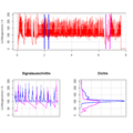
  Welding current of a MAG arc with histograms of signal sections

• 

  Proportions of the ohmic voltage drop in the measured voltage during MIG / MAG welding

• 

  Measured and corrected welding voltage for short arc welding

• 

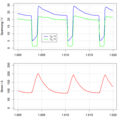
  Measured and corrected welding voltage, welding current for short arc welding

Arc voltage and current monitoring variables

The following explanations describe one of the various options for creating features from process data from MIG / MAG welds and using them for process monitoring.

The signals of the electrical quantities express both the arc energy and the reproducibility of the process.

The voltage drop across the arc and the voltage drop across the free wire length provide different information about the welding process. In the technological environment, only the entire voltage drop over the arc and the free wire length , over the contact tube , over the workpiece and over the welding cable within the voltage tap can be measured together (see figure "Portions of the ohmic voltage drop in the measured voltage with MIG / MAG Welding " ). The inductance of the welding circuit and the resulting inductive component of the measured voltage drop can be neglected for the purposes of process monitoring, as it is low and constant for stationary systems. The measured voltage signal can be interpreted as the sum of the arc voltage and a sum of the various ohmic resistances multiplied by the welding current signal : ${\displaystyle U_{\mathrm {LB} }}$ ${\displaystyle U_{\mathrm {Lf} }}$ ${\displaystyle U_{\mathrm {s} }}$ ${\displaystyle R_{\mathrm {LB} }}$ ${\displaystyle R_{\mathrm {Lf} }}$ ${\displaystyle R_{\mathrm {KR} }}$ ${\displaystyle R_{\mathrm {W} }}$ ${\displaystyle R_{\mathrm {K} }}$ ${\displaystyle R_{\mathrm {sum} }}$ ${\displaystyle i_{\mathrm {s} }}$

${\displaystyle u_{\mathrm {s} }=u_{LB}+R_{\mathrm {sum} }\cdot i_{s}}$ With

${\displaystyle R_{\mathrm {sum} }=R_{\mathrm {Lf} }+R_{\mathrm {KR} }+R_{\mathrm {W} }+R_{\mathrm {K} }}$.

${\displaystyle R_{\mathrm {sum} }}$ is variable due to changes in the temperature conditions of the free wire length, the state of the current contact nozzle, the wire surface and the contact resistance of the workpiece and welding table.

When welding with short-circuit formation ( short arc ), the current-voltage characteristics show different slopes during the short-circuit and burning phases. The gradient in the short-circuit phase represents the voltage drop . If this is known, a corrected welding voltage can be calculated from the measured voltage, which is determined by the arc voltage alone (see pictures "Measured and corrected welding voltage for short arc welding" and "Measured and corrected welding voltage, welding current for short arc welding" ). ${\displaystyle R_{\mathrm {sum} }\cdot i_{s}}$

While the processes in the arc are reflected in the corrected welding voltage, the change in the free wire length and thus the distance between the welding torch and the workpiece surface is expressed in the short circuit voltage. It follows that for process monitoring during welding with short arcs it can be useful to observe the voltage of the arc and burning phases separately. The separation is possible through a voltage threshold below a minimum burning voltage of 14 V.

Characteristics from electrical quantities

Descriptive features of a histogram from the voltage signal during MAG short arc welding

Formation of features from the electrical signals during MAG welding with short arc

The time course of the digitized electrical signals current and voltage can be characterized by empirical frequency distributions (histograms). The descriptive statistics used parameters to the location, scattering, concentration, and shape to describe such distributions. Such parameters are used as features for monitoring. A data record consisting of feature values ​​characterizes the current signal curve and can be understood as a feature pattern. The pictures "Formation of features from the electrical signals during MAG welding with short arc" and "Descriptive features of a histogram ..." illustrate a possible feature formation process:

A time segment of the two voltage signals is considered (left part of the figure). To characterize the shape and position of the density distribution of the current, the parameters “left limit” , “right limit” , “ median ”, “position of the maximum” and “mean value” are calculated (Figure “Descriptive features of a histogram ...” ). The limits on the left and right describe the location of a given percentage of the area under the distribution. A threshold at 14 V divides the voltage into a “burning phase” and “short-circuit phase” . An empirical density is calculated for each sub-area above and below the voltage threshold. From the “short-circuit phase ” only the “median” is used as characteristics, from the “burning phase” the “limits” , the “median” and the “effective value” . To illustrate a feature pattern , the feature values are shown in a radial plot .

Training phase in fusion welding

In the training phase, the target patterns for process monitoring are obtained in a similar way to resistance spot welding (see class formation in the training phase ). Since different welding parameters and different welding positions can be used within a weld seam, different process classes are likely to occur. Each process class has its own target pattern. A monitoring system should automatically recognize the different process classes during the training phase and make separate feature data records available for learning the specific target patterns.

Further physical monitoring quantities and characteristics

Optical signals

The arc temperature and dynamics can be deduced from optical arc information. The image of the interaction between the weld pool and filler metal and the location of the weld pool can also be obtained from this.

Acoustic signals

The sound of the arc provides the arc welder with information about the process stability and the type of droplet transfer.

Importance of online process monitoring in quality assurance

Online process monitoring is part of quality control loop 1 (QRK1) in the quality control loop concept according to Haepp and Hopf. It enables a full test , makes quality control loop 2 largely superfluous and provides data for statistical quality control. It is therefore an essential instrument for quality assurance and permanent process and quality optimization according to the PDCA concept . Information is provided about:

• the current connection quality,
• the current and past process capability and mastery,
• the stability of the manufacturing process over any previous manufacturing period

and it will be

• the necessities of a process intervention,
• the need for process improvement,
• the effectiveness of implemented improvement measures

displayed.

literature

• Yi Ming Zhang: Real-time weld process monitoring. Woodhead Publishing Series in Welding and Other Joining Technologies No. 62, 2008.
• RO Duda, PE Hart, DG Stork: Pattern Classification . 2nd Edition. John Wiley & Sons, 2000, ISBN 0-471-05669-3 .

Individual evidence

1. ^ W. Wiesemann: Process monitoring and closed-loop control. Landolt-Börnstein, New Series VIII / 1C (2001)
2. ↑ ^{a b c} S. F. Bocklisch: Process analysis with fuzzy procedures. Verlag Technik, Berlin 1987, ISBN 3-341-00211-1 .
3. ^ ^{A b} D. Zhou, J. Weston, A. Gretton, O. Bousquet, B. Schölkopf: Ranking on Data Manifolds. 17th Annual Conference on Neural Information Processing Systems (NIPS 2003), MIT Press, Cambridge, MA, pp. 169-176.
4. ^ D. Reynold: Gaussian Mixture Models. ( Memento of the original from August 9, 2017 in the Internet Archive ) Info: The archive link was inserted automatically and has not yet been checked. Please check the original and archive link according to the instructions and then remove this notice. MIT Lincoln Laboratory. 
5. ^ ^{A b} F. Müller, J. Holweg: Method and device for the acquisition and evaluation of process data; Patent EP 1 455 983 B1. 2004.
6. ↑ Spot Welding Joints on Steel Materials - Testing of Body Assemblies Volkswagen AG, PV 6702, 2010.
7. ↑ Kin-ichi Matsuyama: Quality Management of Resistance Welds. IIW-Doc. III-1496-08, 2008.
8. ↑ D. Steinmeier: Resistance Welding - Weld Monitoring Basics-1. microJoining Solutions - microTips
9. ↑ DVS : "Measuring in spot, projection and roll seam welding" , DVS data sheet 2908, 2006.
10. ↑ M. Uran: Quality monitoring for resistance spot welding by means of multi-parametric analysis Quality monitoring for resistance spot welding by means of multi-parameter analysis. Dissertation. TU Berlin 2004, DNB 973319054
11. ^ A. Stiebel: Solution - Thermal Force Feedback (TFF®) system
12. ^ Apparatus and method for monitoring and controlling resistance spot welding. Patent US4419558.
13. ↑ U. Niedergesäß, M. Kraska, M. Berg: Process for ensuring the welding quality of weld spots during resistance spot welding of a certain material combination. Patent DE102008005113.
14. ↑ Welding gun and method for assessing the quality of a welded joint. Patent EP1291113 A1.
15. ↑ M. Janota: Thermal expansion and quality of resistance spot welds. IIW-Doc. III-1479-08, 2008.
16. ↑ SF Bocklisch, J. Burmeister: Method for quality assurance of joining. Patent DD265098A1.
17. ↑ ^{a b} Monitoring system for resistance spot welding, HARMS + WENDE QST GmbH
18. ↑ Igor, W. Merfert: Dynamic improvements on inverter power sources for arc welding with pulsating direct current , Diss., TU Magdeburg 1998, DNB 955255724
19. ↑ Erdmann-Jesnitzer, F .; Rehfeldt, D .: Method and device for monitoring the welding process in electric welding processes, in particular arc and electroslag welding processes , patent of the Swiss Confederation, 1971.
20. ↑ HJ Haepp, B. Hopf: Requirements for a future quality assurance system for laser welding with the remote welding process. In: Laser Magazin. 23 (2006), no.4