
Equilibrium (systems theory)
In the general sense, a system is in equilibrium if it does not change over time without external influence. In the case of dynamic equilibria , only macroscopic changes are generally considered. In a thermodynamic equilibrium , for example, the macrostate of a gas with the state variables pressure , temperature and chemical potential is constant, while the microstate , i.e. the position and speed of individual gas particles, can change.
The state that the system does not leave without external influence is generally called the state of equilibrium , critical point , fixed point , stationary state , equilibrium position . Depending on the context, the terms mentioned are not used synonymously, but contain an additional classification of the state, for example with regard to stability. When considering open systems , an unchanging state is referred to as a “steady state”, while the term “equilibrium” is used for a stationary state after the system has been isolated .
general definition
First, a closed dynamic system is considered . The state of a dynamic system at the point in time can generally be described by a tuple, i.e. an ordered set of all state variables. In order for the state to be a state of equilibrium, it must be the same for all times, one also says "invariant to a dynamic ".


The position and number of states of equilibrium in a system is independent of the state in which the system is, i.e. also independent of whether it is "in equilibrium" or not. The states of equilibrium result as solutions of the equilibrium conditions. Depending on the number of solutions of the equations for the respective equilibrium condition, a system can have any number of equilibrium states.
Continuous dynamic system

For a continuous dynamic system whose time evolution is given by the differential equation

a state of equilibrium is given by the equilibrium condition


since then the time derivative is accordingly . A state of equilibrium is therefore a time-independent solution of the ordinary differential equation or a zero of the function .

Discrete dynamic system

A discrete dynamic system, which only allows discrete time steps, can be represented by an iterated mapping

describe. The equilibrium condition for the state of equilibrium is


The equilibrium point is therefore a time-independent fixed point in the mapping .
State of equilibrium and potential
Instead of looking at the zeros of the function , a potential can be found for many systems , so that it can be written as a negative gradient of the potential. A state of equilibrium then corresponds to an extreme point of the potential. In a thermodynamic system , this is a suitable thermodynamic potential . For example, for a system at constant temperature and pressure, such as a chemical reaction, the Gibbs free enthalpy is suitable , which is minimal when the system is in thermodynamic equilibrium.


In a Hamiltonian system, the state can be described by the position coordinates and impulses . For a state of equilibrium, and . The dynamics are given by the canonical equations . Insertion of the equilibrium condition shows that in a state of equilibrium the partial derivative of the Hamilton function and are zero, the state of equilibrium is therefore an extreme point of the potential.


In mechanics, the location with the coordinates of the equilibrium is also called the position of rest or static position of rest . In particular, a particle does not experience any force in the rest position. “Rest position” is somewhat misleading in this respect: Although there is no force acting on a particle in the rest position, the particle does not have to be at rest there. Only in a static state in which the equilibrium condition is also fulfilled for the impulses is the particle there at rest and the system in equilibrium.
Behavior of equilibria in the event of disturbances
The development of a dynamic system over time can be estimated qualitatively by characterizing the states of equilibrium. A state of equilibrium can be roughly divided into
- stable
- The system returns to its original state after a fault.
- unstable
- The system changes to another state in the event of the slightest disturbance.
- indifferent
- The system comes to rest in a new state after each fault.
- metastable
- After a sufficiently large disturbance, the system changes to a more stable state of equilibrium. In the case of two states of equilibrium, one also speaks of bistable .
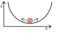
stable equilibrium

unstable equilibrium
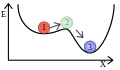
metastable equilibrium

bistable equilibrium

indifferent balance


There are several stability terms in stability theory for the mathematically exact classification . In the following a continuous system is assumed; similar terms can also be defined for systems with discrete time steps.
- Lyapunov stable
- An equilibrium state is Lyapunov stable if a sufficiently small error condition will remain small or precise: For each there is a such that for all times and all trajectories with the following applies: .
- asymptotically stable
- A state of equilibrium is asymptotically stable if it is Lyapunov-stable and attractive, i.e. if it returns to the state of equilibrium in the event of a disturbance. Attractive means that there is one out there, so that each trajectory with all exist and the condition fulfilled.


One method of stability analysis is to linearize the system around the state of equilibrium . With the Hartman-Grobman theorem , the equilibrium state can then be characterized using the eigenvalues of the Jacobi matrix .
Examples
Thermal equilibrium in a house
The time course of the temperature in an unheated house as a function of the outside temperature can be shown in a simple model using the differential equation


describe. The constant is calculated from the area , the heat transfer coefficient of the house walls and the heat capacity of the air. The function on the right side of the equation determines the dynamics of the system. For a state of equilibrium ,


- .

The system has a state of equilibrium at . Because the derivative


is negative, the equilibrium state is stable. If the house is warmer or colder than the surroundings, it cools or warms up until it reaches this state of equilibrium. In this way, by determining the equilibrium points and their stability, statements about the behavior of the system can be made without having to explicitly calculate the temperature curve over time . The integration of the equation, which would be necessary for this explicit calculation, is generally not easy or not analytically possible in non-linear systems.

Mechanical equilibrium in a plane pendulum


A plane pendulum is a mechanical system in which a mass is rotatably attached to a point with a pendulum rod of fixed length . The state of such a pendulum at a fixed point in time can be described by an angle and the angular velocity . The equation of motion is then the autonomous differential equation


where the constant is the gravitational acceleration .

The system thus has two equilibrium points and , which meet the equilibrium condition. The equilibrium point at an angle of zero is the stable equilibrium when the pendulum has no deflection and speed. The second point is the unstable equilibrium when the pendulum has no speed and is "upside down". In phase space there is an elliptical fixed point , the point a hyperbolic fixed point .


In a static system, i.e. a system in which the pendulum has no speed , the condition for mechanical equilibrium can be formulated with the help of forces and moments . The pendulum is in equilibrium when the sum of all acting forces and moments is zero. In both equilibrium points and , the weight of the mass on the pendulum is completely balanced by the force with which the pendulum rod holds the mass at the pivot point. The resulting force and moment are zero.
Ecological balance in a predator-prey relationship

A simple model of the interaction between predator and prey populations is the Lotka-Volterra equations . They describe the development over time of a number of prey animals and predators . With the respective reproduction and death rates or and or , the differential equation system results for a state :


The system has a stable equilibrium point and an unstable equilibrium point . The state has a constant number of predators and prey that are in ecological equilibrium . In the state , both populations are wiped out.


Dynamic equilibria
A system in nature can generally be described in different ways. There are differently detailed possibilities to choose the state variables of the system. In statistical physics, the terms macrostate and microstate are used to differentiate between differently detailed descriptions . In the case of equilibrium considerations, such as a thermodynamic equilibrium, only the macrostate is considered. The system is in equilibrium if the macrostate does not change. However, the microstate of the system can change.
If there are processes within the system or flows across the system boundaries that change the microstate, cancel each other out in their influence on the macrostate of the system, an equilibrium is called dynamic equilibrium or steady state .
Dynamic equilibrium in a closed system
In the case of non-open systems, it is only internal processes that influence the state variables of the system. The equilibrium condition formulated above is fulfilled in systems of chemical reactions exactly when the chemical potentials are balanced. Example: A thermally insulated pressure pot with hot water and steam. The two reactions involved are evaporation and condensation. Evaporation lowers the temperature and increases the pressure, which slows down further evaporation or accelerates condensation. After some time, an equilibrium is established in which both reactions proceed at the same speed and the state variables pressure, temperature and amount of steam remain constant.
For systems in dynamic equilibrium, the virial theorem applies in the respective sub-area of physics. Explicit knowledge of orbits is not required for this.
Quasi-static changes in state
In general, there are more than two reactions that happen at the same time. The equilibrium can then exist between all participating elements of the system or it can be limited to a subsystem. If the processes of the subsystem are fast compared to exchange processes with the environment, then quasi-static changes of state occur. Example: The slowly cooling pressure pot. The release of heat to the environment lowers the temperature, the pressure and the amount of steam, but not independently of one another, rather the system state always remains close to the steam pressure curve .
Whether there is a separation into fast and slow processes in a special case and how the changes in the state variables occur over time is the subject of kinetics .
Fluid equilibria in open systems
If there are several coupling processes with the environment, the state of the system can remain constant in that they cancel each other out more or less randomly. Dynamic equilibria are always associated with the production of entropy , which must be removed for a steady state.
Tight coupling
If a coupling process dominates the other processes, the state of the subsystem is defined in the affected state variable. Examples: The pot is open, the pressure is set to atmospheric pressure, even high heating power does not raise the temperature above the boiling point as long as there is still water in the pot. In electrical engineering, the voltage is fixed ( clamped ) when a small consumer is connected to a voltage source . An economic example is fixed book prices (for works without an alternative, such as special books).
Flow equilibrium in the reaction-free system
Without close coupling, systems will usually react to changes in the environment with significant changes in their state. The term steady state suggests the following example: The level of a tub without stopper is located at a given inflow as level adjustment that the level is dependent on the outflow is equal to the inflow. But there are also constant equilibria with many other physical and non-physical quantities, such as energy or wealth.
Homeostatic balance
The flows across the system boundary can also be balanced out by the system influencing them through internal control processes. The system theory generally calls the subsystem of a complex system that forms the control mechanism homeostat , the prototypical example is the thermostat .
The term homeostasis was coined in connection with living systems in which many system parameters are usually subject to regulation: pH value, osmotic pressure, enzyme concentrations, temperature, number of cells - to name just a few.
Web links
- Eugene M. Izhikevich: Equilibrium Article in Scholarpedia
Individual evidence
- ^ Robert Besancon: The Encyclopedia of Physics . Springer Science & Business Media, 2013, ISBN 1-4615-6902-8 , pp. 406 ( limited preview in Google Book search).
- ^ Rolf Haase: Thermodynamics . Springer-Verlag, 2013, ISBN 3-642-97761-8 , pp. 3 ( limited preview in Google Book Search).
- ^ Steven H. Strogatz : Nonlinear Dynamics and Chaos . Perseus Books Group, 2001; P. 15.
- ↑ Bertram Köhler: Evolution and Entropy Production. Retrieved April 9, 2017 .