Gradient (math)

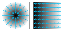
Two scalar fields, shown as a shade of gray (darker color corresponds to a larger function value). The blue arrows on it symbolize the associated gradient.

The gradient as an operator in mathematics generalizes the known gradients that describe the course of physical quantities. As a differential operator , it can be applied to a scalar field and in this case it will yield a vector field called a gradient field . The gradient is a generalization of the derivative in multidimensional analysis . To better differentiate between the operator and the result of its application, such gradients of scalar field sizes are also called gradient vectors in some sources.

In Cartesian coordinates , the components of the gradient vector are the partial derivatives in the point ; the gradient therefore points in the direction of the greatest change. The amount of the gradient indicates the value of the greatest rate of change at that point. ${\displaystyle P}$

If, for example, the relief map of a landscape is interpreted as a function  that assigns the altitude at this point to each location, then the gradient of at that point is a vector that points in the direction of the greatest increase in altitude of . The magnitude of this vector indicates the greatest slope at this point. ${\displaystyle h(x,y),}$ ${\displaystyle h}$ ${\displaystyle (x,y)}$ ${\displaystyle h}$

The gradient is examined together with other differential operators such as divergence and rotation in vector analysis , a sub-area of multidimensional analysis . They are formed with the same vector operator, namely with the Nabla operator (to indicate that the Nabla operator can alternatively be understood as a vector, sometimes also or ). ${\displaystyle \nabla }$ ${\displaystyle {\vec {\nabla }}}$ ${\displaystyle {\underline {\nabla }}}$

definition

On is the scalar product given. The gradient of the totally differentiable function in the point is that due to the requirement ${\displaystyle \mathbb {R} ^{n}}$ ${\displaystyle \langle {\cdot },{\cdot }\rangle }$ ${\displaystyle \operatorname {grad} }$ ${\displaystyle f\colon \mathbb {R} ^{n}\to \mathbb {R} }$ ${\displaystyle a\in \mathbb {R} ^{n}}$

${\displaystyle \mathrm {d} f(a)h=\langle \operatorname {grad} f(a),h\rangle \quad (h\in \mathbb {R} ^{n})}$

uniquely determined vector The operator is the total differential or the Cartan derivative . The definition of the gradient for scalar fields can be extended to vector fields . This generalized gradient is called the vector gradient . ${\displaystyle \operatorname {grad} f(a).}$ ${\displaystyle \mathrm {d} }$ ${\displaystyle f\colon \mathbb {R} ^{n}\to \mathbb {R} }$ ${\displaystyle f\colon \mathbb {R} ^{n}\to \mathbb {R} ^{m}}$

Coordinate representation

The gradient also has different representations in different coordinate systems.

Cartesian coordinates

Im with the standard Euclidean scalar product is the column vector ${\displaystyle \mathbb {R} ^{n}}$ ${\displaystyle \operatorname {grad} f(a)}$

${\displaystyle \operatorname {grad} (f)={\frac {\partial f}{\partial x_{1}}}{\hat {e}}_{1}+\cdots +{\frac {\partial f}{\partial x_{n}}}{\hat {e}}_{n}={\begin{pmatrix}{\frac {\partial f}{\partial x_{1}}}\\\vdots \\{\frac {\partial f}{\partial x_{n}}}\end{pmatrix}}.}$

The entries are the partial derivatives of in -direction. Often one also writes (pronounced “ Nabla ”) instead of Cartesian coordinates . The gradient has the representation in three dimensions ${\displaystyle {\tfrac {\partial f}{\partial x_{i}}}}$ ${\displaystyle f}$ ${\displaystyle x_{i}}$ ${\displaystyle \nabla f}$ ${\displaystyle f}$ ${\displaystyle \operatorname {grad} {f}}$

${\displaystyle \operatorname {grad} (f)=\nabla f={\frac {\partial f}{\partial x}}{\hat {e}}_{x}+{\frac {\partial f}{\partial y}}{\hat {e}}_{y}+{\frac {\partial f}{\partial z}}{\hat {e}}_{z}\,,}$

where , and denote the unit vectors in the direction of the coordinate axes. ${\displaystyle {\hat {e}}_{x}}$ ${\displaystyle {\hat {e}}_{y}}$ ${\displaystyle {\hat {e}}_{z}}$

Calculation example

A scalar field is given by Thus the partial derivatives are and and it follows or in vector representation ${\displaystyle f(x,y)=2x^{2}-y^{2}.}$ ${\displaystyle {\frac {\partial f}{\partial x}}=4x}$ ${\displaystyle {\frac {\partial f}{\partial y}}=-2y}$ ${\displaystyle \operatorname {grad} (f)=\nabla f={\frac {\partial f}{\partial x}}{\hat {e}}_{x}+{\frac {\partial f}{\partial y}}{\hat {e}}_{y}=4x{\hat {e}}_{x}-2y{\hat {e}}_{y}}$ ${\displaystyle \operatorname {grad} (f)=\nabla f={\begin{pmatrix}4x\\-2y\end{pmatrix}}.}$

For example, the gradient vector for the point is . The amount is . ${\displaystyle P(2|1)}$ ${\displaystyle {\begin{pmatrix}8\\-2\end{pmatrix}}}$ ${\displaystyle \left|{\begin{pmatrix}8\\-2\\\end{pmatrix}}\right|={\sqrt {8^{2}+(-2)^{2}}}\approx 8{,}25}$

Cylinder and spherical coordinates

• Representation in three-dimensional cylinder coordinates : ${\displaystyle V=V\left(\rho ;\varphi ;z\right)}$

${\displaystyle \operatorname {grad} V={\frac {\partial V}{\partial \rho }}{\hat {e}}_{\rho }+{\frac {1}{\rho }}{\frac {\partial V}{\partial \varphi }}{\hat {e}}_{\varphi }+{\frac {\partial V}{\partial z}}{\hat {e}}_{z}}$

• Representation in three-dimensional spherical coordinates : ${\displaystyle V=V\left(r;\vartheta ;\varphi \right)}$

${\displaystyle \operatorname {grad} V={\frac {\partial V}{\partial r}}{\hat {e}}_{r}+{\frac {1}{r}}{\frac {\partial V}{\partial \vartheta }}{\hat {e}}_{\vartheta }+{\frac {1}{r\sin \vartheta }}{\frac {\partial V}{\partial \varphi }}{\hat {e}}_{\varphi }}$

These are special cases of the gradient on Riemannian manifolds . For this generalization see: Outer derivative .

Orthogonal coordinates

The gradient is represented in general orthogonal coordinates

${\displaystyle \operatorname {grad} f=\sum _{a}{{\frac {1}{h_{a}}}{\frac {\partial f}{\partial {q_{a}}}}\,{\hat {e}}_{q_{a}}}\,,}$

where they indicate the magnitude and direction of the vector . ${\displaystyle h_{a}}$ ${\displaystyle {\hat {e}}_{q_{a}}}$ ${\displaystyle {\tfrac {\partial {\vec {r}}}{\partial {q_{a}}}}}$

Generally curvilinear coordinates

The gradient is represented in generally curvilinear coordinates

${\displaystyle \operatorname {grad} f=\sum _{a}{\frac {\partial f}{\partial q_{a}}}\,{\vec {G}}^{a}\,,}$

where is the gradient of the coordinate . ${\displaystyle {\vec {G}}^{a}}$ ${\displaystyle q_{a}}$

Coordinate-free representation as a volume derivative

With the help of Gauss's integral theorem , the gradient, like the divergence (source density) and the rotation (vortex density) , can be represented as a volume derivative . This representation has the advantage that it is independent of coordinates. For this reason, the gradient is often defined directly in the field of engineering .

If there is a spatial area with a piecewise smooth edge and the volume, then the gradient of the scalar field in the point can be determined by means of the volume derivative ${\displaystyle {\mathcal {V}}}$ ${\displaystyle \partial {\mathcal {V}}}$ ${\displaystyle V,}$ ${\displaystyle f\colon {\mathcal {V}}\to \mathbb {R} }$ ${\displaystyle p\in {\mathcal {V}}}$

${\displaystyle \operatorname {grad} f=\lim _{V\rightarrow 0}{\frac {\oint _{\partial {\mathcal {V}}}f\,\mathrm {d} {\vec {A}}}{V}}}$

be calculated. In this case, referred to the outer surface vector element of which the outward facing normal vector and the scalar element surface. ${\displaystyle \mathrm {d} {\vec {A}}={\tfrac {\vec {n}}{\mid {\vec {n}}\mid }}\mathrm {d} A}$ ${\displaystyle \partial {\mathcal {V}},}$ ${\displaystyle {\vec {n}}}$ ${\displaystyle \mathrm {d} A}$

To form the limit value, the spatial area is contracted to the point so that its content approaches zero. If you replace with a pressure , the gradient appears as a force density . The coordinate representations of the previous section result from the volume derivation if the respective volume element, for example a sphere or cylinder, is selected as the spatial area . ${\displaystyle {\mathcal {V}}}$ ${\displaystyle P}$ ${\displaystyle V}$ ${\displaystyle f}$ ${\displaystyle {\mathcal {V}}}$

Riemannian manifolds

For a smooth function on a Riemann manifold , the gradient of is that vector field with which for each vector field the equation ${\displaystyle f}$ ${\displaystyle (M,g)}$ ${\displaystyle f}$ ${\displaystyle \nabla f}$ ${\displaystyle X}$

${\displaystyle g(\nabla f,X)=\partial _{X}f,\qquad \mathrm {d.\,h.} \quad g_{x}((\nabla f)_{x},X_{x})=(\partial _{X}f)(x),}$

holds, where the by -defined inner product of tangent to , and (often referred to) that function is associated with each point , the directional derivative of in the direction evaluated in assigns. In other words, in a map from an open subset of to an open subset of is given by: ${\displaystyle g_{x}(\cdot ,\cdot )}$ ${\displaystyle g}$ ${\displaystyle x}$ ${\displaystyle \partial _{X}f}$ ${\displaystyle X(f)}$ ${\displaystyle x\in M}$ ${\displaystyle f}$ ${\displaystyle X}$ ${\displaystyle x}$ ${\displaystyle \varphi }$ ${\displaystyle M}$ ${\displaystyle \mathbb {R} ^{n}}$ ${\displaystyle (\partial _{X}f)(x)}$

${\displaystyle \sum _{j=1}^{n}X^{j}(\varphi (x)){\frac {\partial }{\partial x_{j}}}(f\circ \varphi ^{-1}){\Big |}_{\varphi (x)},}$

where the -th component of in these coordinates means. ${\displaystyle X^{j}}$ ${\displaystyle j}$ ${\displaystyle X}$

The gradient has the form in local coordinates

${\displaystyle \nabla f=g^{ik}{\frac {\partial f}{\partial x^{k}}}{\frac {\partial }{\partial x^{i}}}.}$

Analogous to the case , the relationship between the gradient and the external derivative is mediated ${\displaystyle M=\mathbb {R} ^{n}}$

${\displaystyle (\partial _{X}f)(x)=df_{x}(X_{x})\ .}$

More precisely: is that of the 1-form under the musical isomorphism ("sharp") defined by means of the metric ${\displaystyle \nabla f}$ ${\displaystyle \mathrm {d} f}$ ${\displaystyle g}$

${\displaystyle \sharp =\sharp ^{g}\colon T^{*}M\to TM}$

corresponding vector field. The connection between the external derivative and the gradient for functions on the is the special case for the flat metric given by the Euclidean scalar product. ${\displaystyle \mathbb {R} ^{n}}$

Geometric interpretation

From a geometrical point of view, the gradient of a scalar field at a point is a vector that points in the direction of the steepest rise in the scalar field. The gradient is perpendicular to the level surface ( level set ) of the scalar field in a point . The amount of the vector corresponds to the strength of the increase. If you are at a local minimum or maximum ( extremum ) or at a saddle point , the gradient at this point is precisely the zero vector , provided that this extreme point lies inside the area under consideration. ${\displaystyle P}$

With the help of the gradient, the increase in any direction, called the directional derivative , can also be determined, which - in contrast to the gradient - is again a scalar.

properties

The following applies to all constants and scalar fields : ${\displaystyle c\in \mathbb {R} }$ ${\displaystyle u,\,v\colon \mathbb {R} ^{n}\to \mathbb {R} }$

${\displaystyle \operatorname {grad} c={\vec {0}}}$

Linearity

${\displaystyle \operatorname {grad} (c\cdot u)=c\cdot \operatorname {grad} u}$

${\displaystyle \operatorname {grad} (u+v)=\operatorname {grad} u+\operatorname {grad} v}$

Product rule

${\displaystyle \operatorname {grad} (u\,v)=u\operatorname {grad} v+v\operatorname {grad} u}$

${\displaystyle \operatorname {grad} (u^{n})=nu^{n-1}\ \operatorname {grad} u}$

Relation to the derivation of direction

→ Main article : Directional derivation

The directional derivative means the derivative , i.e. the rise of a scalar field in the direction of a normalized vector : ${\displaystyle \varphi \left({\vec {r}}\right),}$ ${\displaystyle {\vec {v}},}$

${\displaystyle D_{\vec {v}}\varphi ={\frac {\partial \varphi }{\partial {\vec {v}}}}=\lim _{t\to 0}{\frac {\varphi ({\vec {r}}+t{\vec {v}})-\varphi ({\vec {r}})}{t}}}$

If in a neighborhood of is differentiable, then the directional derivative can be calculated as the scalar product of with the gradient of : ${\displaystyle \varphi }$ ${\displaystyle {\vec {r}}}$ ${\displaystyle {\vec {v}}}$ ${\displaystyle \varphi }$

${\displaystyle D_{\vec {v}}\varphi ={\frac {\partial \varphi }{\partial {\vec {v}}}}=\left\langle \operatorname {grad} \varphi ,{\vec {v}}\right\rangle }$

Integrability condition

An important relationship for differentiable gradient fields in dimensions is the statement that these (according to Schwarz's theorem ) are always "integrable" in the following sense: It applies to all and : ${\displaystyle \mathbf {G} (x_{1},\dotsc ,x_{n})=\operatorname {grad} f(x_{1},\dotsc ,x_{n})}$ ${\displaystyle n}$ ${\displaystyle i}$ ${\displaystyle k}$ ${\displaystyle (i,k=1,\dotsc ,n)}$

${\displaystyle {\frac {\partial G_{i}}{\partial x_{k}}}-{\frac {\partial G_{k}}{\partial x_{i}}}\equiv 0}$

This directly verifiable relationship - identical in three dimensions to the freedom of rotation of the field - is necessary for the existence of a "potential function" (more precisely: the function ). The or are the components of the vector field. The integrability condition also implies that the line integral disappears for all closed paths in , which is of great importance in mechanics and electrodynamics. ${\displaystyle f}$ ${\displaystyle \phi =-f}$ ${\displaystyle G_{i}}$ ${\displaystyle G_{k}}$ ${\displaystyle W}$ ${\displaystyle \mathbb {R} ^{n}}$ ${\displaystyle \textstyle \oint _{W}\mathbf {G} \cdot \mathrm {d} \mathbf {r} }$

The reverse also applies locally: the integrability condition

${\displaystyle {\frac {\partial G_{i}}{\partial x_{k}}}-{\frac {\partial G_{k}}{\partial x_{i}}}\equiv 0}$

for a differentiable vector field it is also sufficient for the local existence of a scalar potential function with (cf. total differential # integrability condition ). Under suitable prerequisites for the domain of definition (e.g. star-shaped ) one can even infer the global existence of such a potential function (see Poincaré lemma ). ${\displaystyle \mathbf {G} }$ ${\displaystyle f}$ ${\displaystyle \mathbf {G} (x_{1},\dotsc ,x_{n})=\operatorname {grad} f(x_{1},\dotsc ,x_{n})}$ ${\displaystyle G}$

Useful formulas

The following gradients often occur in physics. The position vector is used. ${\displaystyle {\vec {r}}=r{\hat {e}}_{r}}$

${\displaystyle \operatorname {grad} r={\hat {e}}_{r}={\frac {\vec {r}}{r}}}$

${\displaystyle \operatorname {grad} U(r)={\frac {\partial U}{\partial r}}{\hat {e}}_{r}}$

${\displaystyle \operatorname {grad} {\frac {1}{r}}=-{\frac {1}{r^{2}}}\,\operatorname {grad} r=-{\frac {{\hat {e}}_{r}}{r^{2}}}=-{\frac {\vec {r}}{r^{3}}}}$

${\displaystyle \operatorname {grad} {\frac {1}{|{\vec {r}}-{\vec {r}}^{\,\prime }|}}=-{\frac {1}{|{\vec {r}}-{\vec {r}}^{\,\prime }|^{2}}}\,\operatorname {grad} |{\vec {r}}-{\vec {r}}^{\,\prime }|=-{\frac {{\vec {r}}-{\vec {r}}^{\,\prime }}{|{\vec {r}}-{\vec {r}}^{\,\prime }|^{3}}}}$

Note that in the last example the gradient only acts on and not on . It is therefore also written as. ${\displaystyle {\vec {r}}}$ ${\displaystyle {\vec {r}}^{\prime }}$ ${\displaystyle \nabla _{\vec {r}}}$

Applications

Conservative forces

→ Main article : Conservative force

In physics , many force fields can be represented as the gradient of a potential . Examples are:

a) the gravitational force

${\displaystyle {\vec {F}}_{\mathrm {Gravitation} }(x,y,z)=-m\operatorname {grad} \Phi (x,y,z)\ ,}$

for a central mass M located at the coordinate origin

${\displaystyle {\vec {F}}_{\mathrm {Gravitation} }(r)=-m\operatorname {grad} \Phi (r)=\operatorname {grad} {\frac {GMm}{r}}=-{\frac {GMm}{r^{3}}}\,{\vec {r}}}$

reads

b) or in electrodynamics static electric fields ${\displaystyle {\vec {E}}}$

${\displaystyle {\vec {E}}(x,y,z)=-\operatorname {grad} \phi (x,y,z)\ .}$

Conservative force fields make use of, among other things, that for test masses or test loads, the path integral, the work along any path through the force field is only dependent on the start and end point of the path, but not on its course. ${\textstyle W=\int _{S}{\vec {F}}({\vec {r}})\cdot \mathrm {d} {\vec {r}}}$ ${\displaystyle S}$

Transport phenomena

Numerous transport phenomena can be traced back to the fact that the associated currents can be expressed as a gradient of a scalar field, whereby the proportionality factor that occurs is referred to as the transport coefficient or conductivity.

An example of this is the heat flow in thermodynamics , for the ${\displaystyle {\vec {j}}_{w}}$

${\displaystyle {\vec {j}}_{w}=-\lambda \,\operatorname {grad} T}$

applies, where is the thermal conductivity . ${\displaystyle \lambda }$

In fluid dynamics , a potential flow is understood to be a flow in which the velocities are gradients of a potential. Since the divergence of a gradient vanishes, a conservation law follows from the continuity equation .

Image processing

→ Main article : Edge detection

One problem in image processing is to recognize contiguous areas in an image. Since an image contains discrete values, filters such as the Sobel operator are used to obtain a gradient field of the image. A filter is a matrix that is used to convolve the image (see Discrete Convolution ). The edges in the image can then be recognized as extreme values ​​of the filtered image.

Other uses

• Just as the Gauss-Newton method is used to search for the roots of functions, the gradient method is used for multi-dimensional optimization problems in numerics .
• A pressure gradient microphone uses the pressure differences between spatial points.

Web links

• Pressure gradient and sound velocity are not the same (PDF; 144 kB)
• How do I "bend" Nabla and Delta? - Derivation of the nabla operator for orthonormal curvilinear coordinates on www.matheplanet.com

literature

• Adolf J. Schwab : Conceptual world of field theory. Practical, clear introduction. Electromagnetic fields, Maxwell's equations, gradient, rotation, divergence. 6th, unchanged edition. Springer, Berlin a. a. 2002, ISBN 3-540-42018-5 .
• Konrad Königsberger : Analysis. Volume 2. 4th, revised edition. Springer, Berlin a. a. 2000, ISBN 3-540-43580-8 .

Individual evidence

1. ↑ Ernst Grimsehl : Textbook of Physics. Volume 1: Mechanics, thermodynamics, acoustics. 15th edition, edited by Walter Schallreuter. Teubner, Leipzig 1954, p. 579.
2. ^ Bronstein, Semendjajew, Musiol, Mühlig: Taschenbuch der Mathematik , Verlag Harri Deutsch, Frankfurt, 8th edition 2012, section 13.2, Spatial differential operators