
Fig. 1: Graph of the function


Fig. 2: Graph of the function

Arc tangent and inverse cotangent respectively are two related mathematical Inverse Trigonometric Functions . They are the inverse functions of the suitably restricted tangent and cotangent functions : A restriction of the original domains is necessary because tangent and cotangent are periodic functions . One chooses the interval for the tangent and the interval for the cotangent .![] - \ pi / 2, \ pi / 2 [](https://wikimedia.org/api/rest_v1/media/math/render/svg/43d9c33ca6a3fbfefb8745778f833ddb0b59893b)
![{\ displaystyle] 0, \ pi [}](https://wikimedia.org/api/rest_v1/media/math/render/svg/7f7fa6582460166e2c164b5be01af3bf4a430820)
Together with the arcsine and arcsine as inverse functions of the sine and cosine , the arctangent forms the core of the class of arcsine . Together with the area functions , in the complex function theory they are modifications of the complex logarithm , from which they also inherit the "ambiguity", which in turn derives from the periodicity of the complex exponential function .
Spellings
Mathematical formulas used for the arc tangent as symbols , , , or .
For the arccotangent, the notations and have recently also been used.


Due to the general notation used today for inverse functions , the notation that is widespread on pocket calculators begins to replace the classic notation , which can easily lead to confusion with the reciprocal value of the tangent, the cotangent (see also the notations for the iteration) .

properties
|
|
Arctangent
|
Arccotangent
|
| Domain of definition
|

|
|
|
Image set
|

|

|
|
monotony
|
strictly monotonously increasing
|
strictly falling monotonously
|
|
Symmetries
|
Odd function:

|
Point symmetry too 

|
|
Asymptotes
|
 For For 
|
 for for for for
 
|
|
zeropoint
|

|
no
|
|
Jump points
|
no
|
no
|
|
Poles
|
no
|
no
|
|
Extremes
|
no
|
no
|
|
Turning points
|

|

|
Important functional values
The following table lists the important function values of the two arc functions .

|

|

|

|

|
|

|

|

|

|

|

|

|

|

|

|
|
|

|
|
|
|
|
Other important values are:
|
|
|
|

|

|

|

|

|

|

|

|

|

|

|

|

|

|

|

|
|
|
|
|

|
|
|
|
|

|
|
|
|
|
For tangent values see the formula in the #functional equations section .

Approximate calculation
The following approximations apply:
Arctangent, maximum deviation below 0.005 radians:

CORDIC offers another calculation option .
Arccotangent:

Series development
The Taylor series of the arctangent with the expansion point is:

The Taylor series of the arccotangent with the development point is:

These series converge if and only if and is. To calculate the arctangent for , it can be reduced to an arctangent of arguments with . For this you can either use the functional equation or (to get by without ) the equation


By using this formula multiple times, the amount of the argument can be reduced as desired, which enables a very efficient calculation through the series. After only one application of the above formula, one has an argument with such that the above Taylor series converges, and with each further application it is at least halved, which increases the speed of convergence of the Taylor series with each application of the formula.


Because of the arccotangent at the point of expansion the Taylor series has:


It converges for and there agrees with the principal value given above. It also converges for, however, with the value. Some packets of computer algebra give the main value for the value, which is discontinuous at the origin but point-symmetrical and continuous at the infinitely distant point .


Functional equations
Instead of arguments above 1 or below −1, the arctangent can be derived from arguments between −1 and 1:

-
 .
.
The same applies to the arccotangent:
-
 .
.
When you arrive at an argument (a tangent value) (e.g. by the first replacement) , you can then use the equation
in the case![{\ displaystyle y \ in [0,1]}](https://wikimedia.org/api/rest_v1/media/math/render/svg/75565b2f1c9aa708980c991de7726f71e1e8c556)
![{\ displaystyle \ textstyle y \ in \ left [{\ frac {\ sqrt {3}} {3}}, 1 \ right]}](https://wikimedia.org/api/rest_v1/media/math/render/svg/67c5eca2d608b825cde8094428b930f1ac10c19e)

to use, so with the argument of the arc tangent in each case (now , otherwise ) into the interval with comes to rest.


![{\ displaystyle \ textstyle \ left [0, {\ frac {\ sqrt {3}} {3}} \ right]}](https://wikimedia.org/api/rest_v1/media/math/render/svg/51e7aee0632e3f780d4214efba062dc07ad2b9ba)

More relationships


Because of the point symmetry, there is also a value pair of the arctangent function.


Addition theorems
→ Main article: Addition theorems for arc functions (trigonometry)
The addition theorems for arctangent and arccotangent are obtained with the aid of the addition theorems for tangent and cotangent :


It follows from this in particular for double function values


From the first law you can with

derive the group law for sufficiently small ones. So, for example:


from what

calculated. Furthermore applies

and accordingly

The two equations written as arccotangents:

and

Calculation of the circle number π with the help of the arctangent
The series expansion can be used to calculate the number π with any precision: The simplest formula is the special case, the Leibniz formula

Since it converges extremely slowly (logarithmically) , John Machin used the formula in 1706

to calculate the first 100 decimal places of using the Taylor series for the arctangent. The latter converges faster (linearly) and is still used today for the calculation of .
Over time, more formulas of this type have been found. An example comes from FCW Størmer (1896):

which is equivalent to the fact that the real part and the imaginary part of the Gaussian number
-
 With
With 
are the same.
The same applies to the formula of John Machin, whereby it is about the Gaussian number

goes, which can be calculated with a calculator.
Derivatives
Arctangent:

Arccotangent:

Antiderivatives
Arctangent:
An antiderivative of the arctangent is

Arccotangent:
An antiderivative of the arccotangent is

Complex arctangent and arccotangent
If you allow complex arguments and values, then you have
-

 With
With 
a representation that has already been split up into real and imaginary parts. As is true in real life

With 
In the complex, both the arctangent (as well as the arccotangent) can be expressed by an integral and by the complex logarithm :

for in the double slotted plane
The integral has an integration path which does not cross the imaginary axis except possibly in the unit circle . It's regular and unique in this area .


The arctangent plays an essential role in the symbolic integration of expressions of form

If the discriminant is nonnegative, one can determine an antiderivative by means of partial fraction decomposition . If the discriminant is negative, the expression can be replaced by the substitution


in the form

bring; is an antiderivative

Conversion of flat Cartesian coordinates into polar ones
If a point in the plane is given by polar coordinates , its Cartesian coordinates are given by the equations


|

|

|
certainly.
The conversion in the opposite direction is a little more complicated. In any case, the distance belongs
|
 |

|
of the point from the origin to the solution. Is now then is also and it doesn't matter what value it has. This case is referred to below as the singular case.


But then is because the functions and have the period , determined by the equations only modulo , i.e. i.e. with is also a solution for everyone.


Inverse trigonometric functions are required to get from lengths to angles. Here are two examples where the arctangent is used.
However, the simple arctangent (see Fig. 3) is not sufficient. Because of the periodicity of the tangent of , its definition set must be restricted to a period length of before the inversion , which means that the inverse function (the arctangent) cannot have a larger image set.


Fig. 3: φ as the outer angle of an isosceles triangle
Half angle
In the adjacent Fig. 3, the polar axis (which by definition coincides with the -axis ) is lengthened by the amount in the -direction , i.e. from the pole (and origin) to the point.The triangle is isosceles , so that the angles and are equal. Their sum, i.e. double of one of them, is equal to the outer angle of the triangle. This angle is the polar angle sought with the abscissa point applies in a right-angled triangle


what after resolved
|
 |

|
results. The equation fails when is. Must then due also be. If is now , then it is a singular case. But then the equations are through or fulfilled. This is in line with the amount of images, respectively. the function in the following section.


![{\ displaystyle] - \ pi, + \ pi]}](https://wikimedia.org/api/rest_v1/media/math/render/svg/a182a296d04e5c42b56501224310d834b663be37)

The "arctangent" with two arguments
Another way to achieve a fully-fledged polar angle has been chosen in many programming languages and spreadsheets , namely an extended function that is loaded with the two Cartesian coordinates and that thus has enough information to calculate the polar angle modulo, e.g. in the interval and to be able to return in all four quadrants:

![{\ displaystyle] - \ pi, \ pi],}](https://wikimedia.org/api/rest_v1/media/math/render/svg/8ca06e1f21d227e63285c19448958123dcd970a2)
|
 |

|
Together with the equation , the solutions satisfy the equations :

-
 and
and
-
 ,
,
for with anyone

Arctangent with position parameter
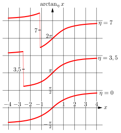
Fig. 4: Arctangent with position parameter
In many applications, the solution to the equation should be as close as possible to a given value . The arctangent function modified
with the parameter is suitable for this


The function rounds to the closest integer.

See also
literature
Web links
References and comments
-
↑ Both functions are monotonous in these intervals, and these are limited by the respective poles .
-
↑ Eric W. Weisstein : Inverse Tangent . In: MathWorld (English).
-
↑ Eric W. Weisstein : Inverse Cotangent . In: MathWorld (English).
-
↑ George Hoever: Higher Mathematics compact . Springer Spectrum, Berlin Heidelberg 2014, ISBN 978-3-662-43994-4 ( limited preview in Google book search).
-
↑ Further approximations (s) ( Memento of 16 April 2009 at the Internet Archive )
-
↑ E.g. the numbers are Størmer numbers ; however not.


-
↑ This is

-
↑ Milton Abramowitz and Irene Stegun : Handbook of Mathematical Functions . (1964) Dover Publications, New York. ISBN 0-486-61272-4 Formula 4.4.3
-
↑ A very similar sketch is that of unit circle # Rationale Parametrisierung .
-
↑ When calculating with floating point numbers, there is instability in the vicinity of the ray because of


