Linear single regression

This scatter diagram shows a concrete empirical regression line of a linear single regression, which was placed as best as possible through the "point cloud" of the measurement.

In statistics , the linear single regression , or also simple linear regression (short: ELR , rarely univariate linear regression ) is a regression analysis method and a special case of linear regression . The term simple indicates that only one independent variable is used in linear single regression to explain the outcome. The aim is to estimate the axis intercept and slope of the regression line as well as to estimate the variance of the disturbance variables .

Introduction to the problem

The goal of a regression is to explain a dependent variable by one or more independent variables. In simple linear regression, a dependent variable is simply explained by an independent variable . The model of linear single regression is therefore based on two metric variables: an influencing variable (also: explanatory variable, regressor or independent variable) and a target variable (also: endogenous variable , dependent variable, declared variable or regressand). In addition, there are pairs of measured values ​​(the representation of the measured values in the - diagram is referred to in the following as a scatter diagram ) which are functionally related, which is composed of a systematic and a stochastic part: ${\displaystyle X}$ ${\displaystyle Y}$ ${\displaystyle n}$ ${\displaystyle (x_{1},y_{1}),\dotsc ,(x_{n},y_{n})}$ ${\displaystyle (x_{1},y_{1}),\dotsc ,(x_{n},y_{n})}$ ${\displaystyle x}$ ${\displaystyle y}$

${\displaystyle Y_{i}=\underbrace {f(x_{i};\beta _{0},\beta _{1},\ldots )} _{\text{systematische Komponente}}+\underbrace {\varepsilon _{i}} _{\text{stochastische Komponente}}}$

The stochastic component describes only random influences (e.g. random deviations such as measurement errors ); all systematic influences are contained in the systematic component. The linear single regression establishes the connection between the influence and the target variable with the help of two fixed, unknown, real parameters and in a linear way, i.e. H. the regression function is specified as follows : ${\displaystyle \beta _{0}}$ ${\displaystyle \beta _{1}}$ ${\displaystyle f(\cdot )}$

${\displaystyle f(x_{i};\beta _{0},\beta _{1})=\beta _{0}+\beta _{1}x_{i}}$( Linearity )

This results in the model of simple linear regression as follows: . Here is the dependent variable and represents a random variable . The values ​​are observable, non-random measured values ​​of the known explanatory variables ; the parameters and are unknown scalar regression parameters and is a random and unobservable disturbance variable. In simple linear regression, a straight line is drawn through the scatter plot in such a way that the linear relationship between and is described as well as possible. ${\displaystyle Y_{i}=\beta _{0}+\beta _{1}x_{i}+\varepsilon _{i}}$ ${\displaystyle Y_{i}}$ ${\displaystyle x_{i}}$ ${\displaystyle x}$ ${\displaystyle \beta _{0}}$ ${\displaystyle \beta _{1}}$ ${\displaystyle \varepsilon _{i}}$ ${\displaystyle X}$ ${\displaystyle Y}$

Introductory example

A well-known sparkling wine producer wants to bring a high-quality Riesling sparkling wine to market. To determine the sales price , a price-sales function should first be determined. For this purpose, a test sale is carried out in shops and you get six value pairs with the respective retail price of a bottle (in euros) and the number of bottles sold : ${\displaystyle n=6}$ ${\displaystyle x}$ ${\displaystyle y}$

business ${\displaystyle i}$	1	2	3	4th	5	6th
Bottle price ${\displaystyle x_{i}}$	20th	16	15th	16	13	10
sold amount ${\displaystyle y_{i}}$	0	3	7th	4th	6th	10

Estimated regression coefficients
${\displaystyle {\begin{aligned}{\hat {\beta }}_{1}&={\frac {\sum \nolimits _{i=1}^{n}(x_{i}-{\overline {x}})(y_{i}-{\overline {y}})}{\sum \nolimits _{i=1}^{n}(x_{i}-{\overline {x}})^{2}}}\\{\hat {\beta }}_{0}&={\overline {y}}-{\hat {\beta }}_{1}{\overline {x}}\end{aligned}}}$
Symbols used
${\displaystyle {\overline {x}}}$, ${\displaystyle {\overline {y}}}$	Mean of the measured values
${\displaystyle x_{i}}$, ${\displaystyle y_{i}}$	Readings

If one looks at the above scatter diagram, one can assume that there is a linear relationship. There you can see that the entered data points are almost on a line. Furthermore, the price is defined as an independent variable and the number of bottles sold as a dependent variable and there are six observations. The number of bottles sold may not only depend on the price, e.g. B. could have hung a large billboard in the sales point 3, so that more bottles were sold there than expected (coincidental influence). So the simple linear regression model seems to fit.

After the graphical inspection of whether there is a linear relationship, the regression line is first estimated using the least squares method and the formulas in the info box for the estimated regression parameters result .

A result of the following numerical example for the dependent and independent variables each mean to and . Thus, the estimated values for and for are obtained by simply inserting them into the formulas explained below. Intermediate values ​​(e.g. ) in these formulas are shown in the following table ${\displaystyle {\overline {x}}=15}$ ${\displaystyle {\overline {y}}=5}$ ${\displaystyle {\hat {\beta }}_{0}}$ ${\displaystyle \beta _{0}}$ ${\displaystyle {\hat {\beta }}_{1}}$ ${\displaystyle \beta _{1}}$ ${\displaystyle \ {\hat {\varepsilon }}_{i}=y_{i}-{\hat {y}}_{i}}$

${\displaystyle \ i}$	Bottle price ${\displaystyle \ x_{i}}$	sold amount ${\displaystyle \ y_{i}}$	${\displaystyle \ (x_{i}-{\overline {x}})}$	${\displaystyle \ (y_{i}-{\overline {y}})}$	${\displaystyle \ (x_{i}-{\overline {x}})(y_{i}-{\overline {y}})}$	${\displaystyle (x_{i}-{\overline {x}})^{2}}$	${\displaystyle (y_{i}-{\overline {y}})^{2}}$	${\displaystyle \ {\hat {y}}_{i}}$	${\displaystyle \ {\hat {\varepsilon }}_{i}}$	${\displaystyle \ {\hat {\varepsilon }}_{i}^{2}}$
1	20th	0	5	−5	−25	25th	25th	0.09	−0.09	0.0081
2	16	3	1	−2	−2	1	4th	4.02	−1.02	1.0404
3	15th	7th	0	2	0	0	4th	5.00	2.00	4.0000
4th	16	4th	1	−1	−1	1	1	4.02	−0.02	0.0004
5	13	6th	−2	1	−2	4th	1	6.96	−0.96	0.9216
6th	10	10	−5	5	−25	25th	25th	9.91	0.09	0.0081
total	90	30th	0	0	−55	56	60	30.00	0.00	5.9786

It results in the example

${\displaystyle {\hat {\beta }}_{1}={\frac {\sum \nolimits _{i=1}^{6}(x_{i}-{\overline {x}})(y_{i}-{\overline {y}})}{\sum \nolimits _{i=1}^{6}(x_{i}-{\overline {x}})^{2}}}={\frac {-55}{56}}=-0{,}98\quad }$and . ${\displaystyle \quad {\hat {\beta }}_{0}={\overline {y}}-{\hat {\beta }}_{1}{\overline {x}}=5-(-0{,}98)\cdot 15=19{,}73}$

The estimated regression line is thus

${\displaystyle {\hat {y}}_{i}=19{,}73-0{,}98x_{i}}$,

so that one can assume that for every euro more, sales decrease by about one bottle on average.

The sales volume can be calculated for a specific price , e.g. B. results in an estimated sales volume of . An estimated sales volume can be specified for each observation value, e.g. B. for results . The estimated disturbance variable, called the residual , is then . ${\displaystyle x}$ ${\displaystyle x=11}$ ${\displaystyle {\hat {y}}=19{,}73-0{,}98\cdot 11=8{,}93}$ ${\displaystyle x_{i}}$ ${\displaystyle x_{3}=15}$ ${\displaystyle {\hat {y}}_{3}=19{,}73-0{,}98\cdot 15=5}$ ${\displaystyle {\hat {\varepsilon }}_{3}=y_{3}-{\hat {y}}_{3}=7-5=2{,}00}$

Coefficient of determination

→ Main article : coefficient of determination

Scatter plot of residuals with no structure that yields ${\displaystyle R^{2}=0}$

Scatter plot of the residuals that a near gives ${\displaystyle R^{2}}$ ${\displaystyle 1}$

The coefficient of determination measures how well the measured values to a regression model fit ( goodness ). It is defined as the proportion of the " explained variation " in the " total variation " and is therefore between: ${\displaystyle R^{2}=1-SQR/SQT}$

• ${\displaystyle 0\,\%}$(or ): no linear relationship and ${\displaystyle 0}$
• ${\displaystyle 100\,\%}$(or ): perfect linear relationship. ${\displaystyle 1}$

The closer the coefficient of determination is to the value one, the higher the “specificity” or “quality” of the adjustment. Is , then the “best” linear regression model consists only of the intercept while is. The closer the value of the coefficient of determination is, the better the regression line explains the true model . If , then the dependent variable can be fully explained by the linear regression model. The measurement points then clearly lie on the non-horizontal regression line. In this case, there is no stochastic relationship, but a deterministic one. ${\displaystyle R^{2}=0}$ ${\displaystyle {\hat {\beta }}_{0}}$ ${\displaystyle {\hat {\beta }}_{1}=0}$ ${\displaystyle 1}$ ${\displaystyle R^{2}=1}$ ${\displaystyle Y}$ ${\displaystyle (x_{1},y_{1}),\ldots ,(x_{n},y_{n})}$

A common misinterpretation of a low coefficient of determination is that there is no connection between the variables. In fact, only the linear relationship is measured, i.e. H. although is small, there can still be a strong nonlinear relationship. Conversely, a high value of the coefficient of determination does not have to mean that a nonlinear regression model is not even better than a linear model. ${\displaystyle R^{2}}$

In a simple linear regression, the coefficient of determination corresponds to the square of the Bravais-Pearson correlation coefficient (see coefficient of determination as a squared correlation coefficient ). ${\displaystyle R^{2}}$ ${\displaystyle r_{xy}}$

In the above example, the quality of the regression model can be checked with the aid of the coefficient of determination . For the example we get the residual sum of squares and the total sum of squares

${\displaystyle SQR=\sum _{i=1}^{6}(y_{i}-{\hat {y}}_{i})^{2}=5{,}98\quad }$ and ${\displaystyle \quad SQT=\sum _{i=1}^{6}(y_{i}-{\overline {y}})^{2}=60}$

and the coefficient of determination

${\displaystyle R^{2}=1-{\frac {\displaystyle \sum \nolimits _{i=1}^{6}(y_{i}-{\hat {y}}_{i})^{2}}{\displaystyle \sum \nolimits _{i=1}^{6}(y_{i}-{\overline {y}})^{2}}}=1-{\frac {5{,}98}{60}}=0{,}90}$.

This means that approx. 90% of the variation or scatter in can be "explained" with the help of the regression model, only 10% of the scatter remains "unexplained". ${\displaystyle Y}$

The model

Data set with true regression line (blue) and estimated regression line (red) as well as true disturbance variable and estimated disturbance variable (residual).

In the regression model, the random components are modeled with the help of random variables . If is a random variable, then it is too . The observed values are interpreted as realizations of the random variables . ${\displaystyle \varepsilon _{i}}$ ${\displaystyle \varepsilon _{i}}$ ${\displaystyle Y_{i}}$ ${\displaystyle y_{i}}$ ${\displaystyle Y_{i}}$

This results in the simple linear regression model:

${\displaystyle Y_{i}=\beta _{0}+\beta _{1}\ x_{i}+\varepsilon _{i},\quad i=1,\dotsc ,n}$(with random variables ) or

${\displaystyle y_{i}=\beta _{0}+\beta _{1}\ x_{i}+\varepsilon _{i},\quad i=1,\dotsc ,n}$ (with their realizations).

Figuratively speaking, a straight line is drawn through the scatter plot of the measurement. In the current literature, the straight line is often described by the axis intercept and the slope parameter. The dependent variable is often called the endogenous variable in this context. There is an additive stochastic disturbance variable that measures deviations from the ideal relationship - i.e. the straight line - parallel to the axes. ${\displaystyle \beta _{0}}$ ${\displaystyle \beta _{1}}$ ${\displaystyle \varepsilon _{i}}$

The regression parameters and are estimated on the basis of the measured values . This is how the sample regression function is obtained . In contrast to the independent and dependent variables, the random components and their realizations are not directly observable. Their estimated realizations are only indirectly observable and are called residuals . They are calculated quantities and measure the vertical distance between the observation point and the estimated regression line ${\displaystyle (x_{1},y_{1}),\dotsc ,(x_{n},y_{n})}$ ${\displaystyle \beta _{0}}$ ${\displaystyle \beta _{1}}$ ${\displaystyle {\hat {y}}={\hat {\beta }}_{0}+{\hat {\beta }}_{1}x}$ ${\displaystyle \varepsilon _{i}}$ ${\displaystyle {\hat {\varepsilon }}_{i}}$

Model assumptions

In order to ensure the decomposition of into a systematic and random component and to have good estimation properties for the estimation and the regression parameters and , some assumptions regarding the disturbance variables and the independent variable are necessary. ${\displaystyle Y_{i}}$ ${\displaystyle {\hat {\beta }}_{0}}$ ${\displaystyle {\hat {\beta }}_{1}}$ ${\displaystyle \beta _{0}}$ ${\displaystyle \beta _{1}}$

Assumptions about the independent variable

With regard to the independent variable, the following assumptions are made:

The values ​​of the independent variables are deterministic, ie they are fixed ${\displaystyle x_{i}}$

They can therefore be controlled like in an experiment and are therefore not random variables ( exogeneity of the regressors ). If the random variables, e.g. B. if they can only be measured with errors, then the distribution of and the distribution parameters ( expected value and variance) would not only depend on ${\displaystyle x_{i}}$ ${\displaystyle x_{i}}$ ${\displaystyle Y_{i}=\beta _{0}+\beta _{1}X_{i}+\varepsilon _{i}}$ ${\displaystyle Y_{i}}$ ${\displaystyle \varepsilon _{i}}$

${\displaystyle \operatorname {E} (Y_{i})=\beta _{0}+\beta _{1}\operatorname {E} (X_{i})+\operatorname {E} (\varepsilon _{i})}$.

This case can also be treated with special regression methods, see e.g. B. Regression with stochastic regressors .

Sample variation in the independent variable

The realizations of the independent variables are not all the same. So one rules out the unlikely case that the independent variable shows no variability; H. . This implies that the sum of squares of the independent variable must be positive. This assumption is required in the estimation process. ${\displaystyle x_{1},\ldots ,x_{n}}$ ${\displaystyle x_{1}=x_{2}=\ldots =x_{n}={\overline {x}}}$ ${\displaystyle \sum \nolimits _{i=1}^{n}(x_{i}-{\overline {x}})^{2}}$

Assumptions about the independent and dependent variable

The true relationship between the variables and is linear ${\displaystyle x_{i}}$ ${\displaystyle y_{i}}$

The regression equation of simple linear regression must be linear in the parameters and , but can include nonlinear transformations of the independent and dependent variables. For example the transformations ${\displaystyle \beta _{0}}$ ${\displaystyle \beta _{1}}$

${\displaystyle \log(y_{i})=\beta _{0}+\beta _{1}\log(x_{i})+\varepsilon _{i}\quad }$ and ${\displaystyle \quad y_{i}=\beta _{0}+\beta _{1}{\frac {x_{i1}+x_{i2}}{2}}+\varepsilon _{i}}$

permissible because they also represent linear models . Note that transformed data changes the interpretation of the regression parameters.

Presence of a random sample

There is a random sample of the scope with realizations that follows the true model . ${\displaystyle n}$ ${\displaystyle (X_{1},Y_{1}),\ldots ,(X_{n},Y_{n})}$ ${\displaystyle (x_{1},y_{1}),\ldots ,(x_{n},y_{n})}$ ${\displaystyle y_{i}=\beta _{0}+\beta _{1}x_{i}+\varepsilon _{i}}$

Assumptions about the disturbance variables

The following assumptions are made with regard to the disturbance variables:

The expected value of the disturbance variables is zero:

If the model contains an axis intercept that differs from zero, it is reasonable to require at least that the mean value of in the population is zero and that the fluctuations of the individual disturbance variables balance out over the entirety of the observations. Mathematically, this means that the expected value of the disturbance variables is zero . This assumption does not make a statement about the relationship between and , but only makes a statement about the distribution of the unsystematic component in the population. This means that the model under consideration corresponds on average to the true relationship. If the expected value were not zero, then on average one would estimate a wrong relationship. This assumption can be violated if a relevant variable is not taken into account in the regression model (see bias due to omitted variables ). ${\displaystyle \varepsilon _{i}}$ ${\displaystyle \operatorname {E} (\varepsilon _{i})=0\quad ,i=1,\ldots ,n}$ ${\displaystyle x}$ ${\displaystyle \varepsilon }$

The disturbance variables are mutually independent random variables ${\displaystyle \varepsilon _{i},\dotsc ,\varepsilon _{n}}$

If the disturbance variables were not independent, one could formulate a systematic relationship between them. That would contradict breaking down into a clear systematic and random component. In the time series analysis, e.g. B. is often considered a connection of form . ${\displaystyle Y}$ ${\displaystyle \varepsilon _{i}=f(\varepsilon _{i-1},\varepsilon _{i-2},\ldots )}$

Often only the uncorrelatedness of the disturbance variables is required: or equivalent . ${\displaystyle \operatorname {Cov} (\varepsilon _{i},\varepsilon _{j})=\operatorname {E} [(\varepsilon _{i}-\operatorname {E} (\varepsilon _{i}))((\varepsilon _{j}-\operatorname {E} (\varepsilon _{j}))]=\operatorname {E} (\varepsilon _{i}\varepsilon _{j})=0\quad \forall i\neq j,\;i=1,\ldots ,n,\;j=1,\ldots ,n}$ ${\displaystyle \operatorname {Cov} (Y_{i},Y_{j})=0}$

Independent random variables are always also uncorrelated. In this context, one speaks of the absence of autocorrelation .

A constant variance ( homoscedasticity ) of the disturbance variables: ${\displaystyle \forall i:\operatorname {Var} (\varepsilon _{i})=\operatorname {Var} (Y_{i})=\sigma ^{2}=\mathrm {konst.} }$

If the variance were not constant, the variance could possibly be modeled systematically, i. H. this would contradict the decomposition of into a clear systematic and random component. It can also be shown that the estimation properties of the regression parameters can be improved if the variance is not constant. ${\displaystyle Y_{i}}$

All of the above assumptions about the disturbance variables can be summarized as follows:

${\displaystyle \varepsilon _{i}\;{\stackrel {\mathrm {u.i.v.} }{\sim }}\;(0,\sigma ^{2})\quad ,i=1,\ldots ,n}$,

d. H. all disturbance variables are independent and identically distributed with expected value and . ${\displaystyle \operatorname {E} (\varepsilon _{i})=0}$ ${\displaystyle \operatorname {Var} (\varepsilon _{i})=\sigma ^{2}}$

Optional assumption: the disturbance variables are normally distributed , i.e. ${\displaystyle \varepsilon _{i}\;\sim \;{\mathcal {N}}(0,\sigma ^{2})\quad ,i=1,\ldots ,n}$

This assumption is only needed to e.g. B. to calculate confidence intervals or to perform tests for the regression parameters.

If the normal distribution of the disturbance variables is assumed, it follows that the following is also normal: ${\displaystyle Y_{i}}$

${\displaystyle Y_{i}\;\sim \;{\mathcal {N}}\left(\operatorname {E} (Y_{i}),\operatorname {Var} (Y_{i})\right)}$

The distribution of the depends on the distribution of the disturbance variables. The expected value of the dependent variable is: ${\displaystyle Y_{i}}$

${\displaystyle \operatorname {E} (Y_{i})=\operatorname {E} \left(\beta _{0}+\beta _{1}x_{i}+\varepsilon _{i}\right)=\beta _{0}+\beta _{1}x_{i}}$

Since the only random component in the disturbance is the variance of the dependent variable, it is equal to the variance of the disturbance: ${\displaystyle Y_{i}}$ ${\displaystyle \varepsilon _{i}}$

${\displaystyle \operatorname {Var} (Y_{i})=\operatorname {Var} (\beta _{0}+\beta _{1}x_{i}+\varepsilon _{i})=\operatorname {Var} (\varepsilon _{i})=\sigma ^{2}}$.

The variance of the disturbance variables thus reflects the variability of the dependent variables around their mean value. This results in the distribution of the dependent variables:

${\displaystyle Y_{i}\;\sim \;{\mathcal {N}}\left(\beta _{0}+\beta _{1}x_{i},\sigma ^{2}\right)}$.

Based on the assumption that the disturbance variables must be zero on average, the expected value of the regression function of the population must be ${\displaystyle Y_{i}}$

${\displaystyle y_{i}=\beta _{0}+\beta _{1}x_{i}}$

correspond. I.e. with the assumption about the disturbance variables one concludes that the model has to be correct on average. If, in addition to the other assumptions, the assumption of normal distribution is also required, one also speaks of the classical linear model (see also #Classical linear model of normal regression ).

As part of the regression diagnosis , the requirements of the regression model should be checked as far as possible. This includes checking whether the disturbance variables have no structure (which would then not be random).

Estimation of the regression parameters and the confounding variables

The estimation of the regression parameters and the disturbance variables takes place in two steps: ${\displaystyle \beta _{0}}$ ${\displaystyle \beta _{1}}$ ${\displaystyle \varepsilon _{i}}$

1. First of all, the unknown regression parameters and are estimated with the help of least squares estimation . The sum of the squared deviations between the estimated regression value and the observed value is minimized. The following formulas result: ${\displaystyle \beta _{0}}$ ${\displaystyle \beta _{1}}$ ${\displaystyle {\hat {y}}_{i}={\hat {\beta }}_{0}+{\hat {\beta }}_{1}x_{i}}$ ${\displaystyle y_{i}}$

   ${\displaystyle {\hat {\beta }}_{1}={\frac {\sum \nolimits _{i=1}^{n}(x_{i}-{\overline {x}})(y_{i}-{\overline {y}})}{\sum \nolimits _{i=1}^{n}(x_{i}-{\overline {x}})^{2}}}={\frac {SP_{xy}}{SQ_{x}}}}$

   ${\displaystyle {\hat {\beta }}_{0}={\overline {y}}-{\hat {\beta }}_{1}{\overline {x}}}$

2. If and are calculated, the residual can be estimated as . ${\displaystyle {\hat {\beta }}_{0}}$ ${\displaystyle {\hat {\beta }}_{1}}$ ${\displaystyle {\hat {\varepsilon }}_{i}=y_{i}-{\hat {y}}_{i}=y_{i}-{\hat {\beta }}_{0}-{\hat {\beta }}_{1}x_{i}}$

Derivation of the formulas for the regression parameters

Least Squares Method: The sum of the blue squares of differences is the total sum of squares and the sum of the red squares is the sum of squares of residuals . The least squares estimates and minimize the sum of the squares of the perpendicular distances of the data points from the regression line. ${\displaystyle b_{0}}$ ${\displaystyle b_{1}}$

In order to determine the parameters of the straight line, the objective function ( sum of squares of errors or the sum of squares of residuals ) is minimized ${\displaystyle Q}$

${\displaystyle \left({\hat {\beta }}_{0},{\hat {\beta }}_{1}\right)={\underset {\beta _{0},\beta _{1}\in \mathbb {R} }{\arg \min }}\,Q(\beta _{0},\beta _{1})={\underset {\beta _{0},\beta _{1}\in \mathbb {R} }{\arg \min }}\sum _{i=1}^{n}\left(y_{i}-(\beta _{0}+\beta _{1}x_{i})\right)^{2}}$

The first order conditions ( necessary conditions ) are:

${\displaystyle \left.{\frac {\partial \,Q(\beta _{0},\,\beta _{1})}{\partial \beta _{0}}}\right|_{{\hat {\beta }}_{0}}=-2\sum _{i=1}^{n}\left(y_{i}-{\hat {\beta }}_{0}-\beta _{1}x_{i}\right){\overset {\mathrm {!} }{=}}\;0\quad }$

and

${\displaystyle \left.{\frac {\partial \,Q(\beta _{0},\,\beta _{1})}{\partial \beta _{1}}}\right|_{{\hat {\beta }}_{1}}=-2\sum _{i=1}^{n}x_{i}\left(y_{i}-\beta _{0}-{\hat {\beta }}_{1}x_{i}\right){\overset {\mathrm {!} }{=}}\;0}$.

By setting the partial derivatives according to and to zero, the parameter estimates we are looking for are obtained , for which the sum of the squares of the residuals is minimal: ${\displaystyle \beta _{0}}$ ${\displaystyle \beta _{1}}$

${\displaystyle {\hat {\beta }}_{1}={\frac {\sum \nolimits _{i=1}^{n}(x_{i}-{\overline {x}})(y_{i}-{\overline {y}})}{\sum \nolimits _{i=1}^{n}(x_{i}-{\overline {x}})^{2}}}={\frac {SP_{xy}}{SQ_{x}}}\;}$and , ${\displaystyle \;{\hat {\beta }}_{0}={\overline {y}}-{\hat {\beta }}_{1}{\overline {x}}}$

wherein the sum of differential products between and and the sum of squares of representing. With the aid of Steiner's theorem of displacement , the following can also be represented more simply, in a non- centered form ${\displaystyle SP_{xy}}$ ${\displaystyle x}$ ${\displaystyle y}$ ${\displaystyle SQ_{x}}$ ${\displaystyle x}$ ${\displaystyle {\hat {\beta }}_{1}}$

${\displaystyle {\hat {\beta }}_{1}={\frac {\sum _{i=1}^{n}(x_{i}y_{i})-n{\overline {x}}{\overline {y}}}{\left(\sum _{i=1}^{n}x_{i}^{2}\right)-n{\overline {x}}^{2}}}}$.

Further representations of can be obtained by writing the formula as a function of the Bravais-Pearson correlation coefficient . Either as ${\displaystyle {\hat {\beta }}_{1}}$ ${\displaystyle r_{xy}}$

${\displaystyle {\hat {\beta }}_{1}={\frac {{\sqrt {\displaystyle \sum \nolimits _{i=1}^{n}\left(x_{i}-{\bar {x}}\right)^{2}}}{\sqrt {\displaystyle \sum \nolimits _{i=1}^{n}\left(y_{i}-{\bar {y}}\right)^{2}}}}{\displaystyle \sum \nolimits _{i=1}^{n}\left(x_{i}-{\bar {x}}\right)^{2}}}r_{xy}\;}$or , ${\displaystyle \;{\hat {\beta }}_{1}=r_{xy}{\frac {s_{y}}{s_{x}}}}$

where and represent the empirical standard deviations of and . The latter representation implies that the least squares estimator for the slope is proportional to the Bravais-Pearson correlation coefficient , ie . ${\displaystyle s_{x}}$ ${\displaystyle s_{y}}$ ${\displaystyle x}$ ${\displaystyle y}$ ${\displaystyle r_{xy}}$ ${\displaystyle {\hat {\beta }}_{1}\propto r_{xy}}$

The respective least squares estimates of and are abbreviated as and . ${\displaystyle {\hat {\beta }}_{0}}$ ${\displaystyle {\hat {\beta }}_{1}}$ ${\displaystyle b_{0}}$ ${\displaystyle b_{1}}$

Algebraic Properties of Least Squares Estimators

Three properties can be derived from the formulas:

1.) The regression line runs through the center of gravity or through the "center of gravity" of the data , which follows directly from the definition of above . It should be noted that this only applies if an intercept is used for the regression, as can easily be seen in the example with the two data points . ${\displaystyle ({\overline {x}},{\overline {y}})}$ ${\displaystyle {\hat {\beta }}_{0}}$ ${\displaystyle (x_{1},y_{1})=(1,0),(x_{2},y_{2})=(2,1)}$

2.) The KQ regression line is determined in such a way that the residual sum of squares becomes a minimum. Equivalently, this means that positive and negative deviations from the regression line cancel each other out. If the model of linear single regression contains an intercept that differs from zero, then it must be true that the sum of the residuals is zero (this is equivalent to the property that the averaged residuals result in zero)

${\displaystyle \sum _{i=1}^{n}{\hat {\varepsilon }}_{i}=0}$or . ${\displaystyle {\overline {\hat {\varepsilon }}}={\frac {1}{n}}\sum _{i=1}^{n}{\hat {\varepsilon }}_{i}=0}$

Or, as the residuals as a function of interference can be displayed . This representation is required for the derivation of the unbiased estimate of the variance of the disturbance variables . ${\displaystyle {\overline {\hat {\varepsilon }}}={\overline {\varepsilon }}-({\hat {\beta }}_{0}-\beta _{0})-({\hat {\beta }}_{1}-\beta _{1}){\overline {x}}=0}$

3.) The residuals and the independent variables are (regardless of whether an axis intercept was included or not) uncorrelated, i. H.

${\displaystyle \sum _{i=1}^{n}x_{i}{\hat {\varepsilon }}_{i}=0}$, which follows directly from the second optimality condition above.

The residuals and the estimated values ​​are uncorrelated; H.

${\displaystyle \sum _{i=1}^{n}{\hat {\varepsilon }}_{i}{\hat {y}}_{i}=0}$.

This uncorrelation of the predicted values ​​with the residuals can be interpreted in such a way that all relevant information of the explanatory variables with regard to the dependent variables is already contained in the prediction.

Estimator functions of the least squares estimator

The estimation functions for and for can be derived from the regression equation. ${\displaystyle y_{i}=\beta _{0}+\beta _{1}x_{i}+\varepsilon _{i}}$ ${\displaystyle {\hat {\beta }}_{1}}$ ${\displaystyle \beta _{1}}$ ${\displaystyle {\hat {\beta }}_{0}}$ ${\displaystyle \beta _{0}}$

${\displaystyle {\hat {\beta }}_{1}={\frac {\sum \nolimits _{i=1}^{n}(x_{i}-{\overline {x}})(Y_{i}-{\overline {Y}})}{\sum \nolimits _{i=1}^{n}(x_{i}-{\overline {x}})^{2}}}=\sum \nolimits _{i=1}^{n}w_{i}Y_{i}-{\overline {Y}}\underbrace {\sum \nolimits _{i=1}^{n}w_{i}} _{=0}}$ with the weight function ${\displaystyle w_{i}=w_{i}(x_{i})={\frac {(x_{i}-{\overline {x}})}{\sum \nolimits _{j=1}^{n}(x_{j}-{\overline {x}})^{2}}}}$

${\displaystyle {\hat {\beta }}_{0}={\overline {Y}}-{\hat {\beta }}_{1}{\overline {x}}=\sum \nolimits _{i=1}^{n}({\tfrac {1}{n}}-{\overline {x}}w_{i})Y_{i}}$.

The formulas also show that the estimators of the regression parameters depend linearly on. Assuming a normal distribution of the residuals (or if, for the central limit theorem is satisfied), it follows that also the estimation functions of the regression parameters , and are at least approximate a normal distribution: ${\displaystyle Y_{i}}$ ${\displaystyle \varepsilon _{i}\sim {\mathcal {N}}(0,\sigma ^{2})}$ ${\displaystyle Y_{i}}$ ${\displaystyle {\hat {\beta }}_{1}}$ ${\displaystyle {\hat {\beta }}_{0}}$

${\displaystyle {\hat {\beta }}_{1}\;{\stackrel {a}{\sim }}\;{\mathcal {N}}(\beta _{1},\sigma _{{\hat {\beta }}_{1}}^{2})}$and . ${\displaystyle {\hat {\beta }}_{0}\;{\stackrel {a}{\sim }}\;{\mathcal {N}}(\beta _{0},\sigma _{{\hat {\beta }}_{0}}^{2})}$

Statistical Properties of Least Squares Estimators

Unexpected least squares estimator

The estimators of the regression parameters and are fair to expectation for and , i.e. H. it applies and . The least squares estimator therefore delivers the true values ​​of the coefficients “on average” . ${\displaystyle {\hat {\beta }}_{1}}$ ${\displaystyle {\hat {\beta }}_{0}}$ ${\displaystyle \beta _{1}}$ ${\displaystyle \beta _{0}}$ ${\displaystyle \operatorname {E} ({\hat {\beta }}_{1})=\beta _{1}}$ ${\displaystyle \operatorname {E} ({\hat {\beta }}_{0})=\beta _{0}}$

By linearity of expectation and requirement follows namely and: . The expected value of is therefore: ${\displaystyle \operatorname {E} (\varepsilon _{i})=0}$ ${\displaystyle \operatorname {E} (Y_{i})=\beta _{0}+\beta _{1}x_{i}}$ ${\displaystyle \operatorname {E} ({\overline {Y}})=\beta _{0}+\beta _{1}{\overline {x}}}$ ${\displaystyle {\hat {\beta }}_{1}}$

${\displaystyle {\begin{aligned}\operatorname {E} ({\hat {\beta }}_{1})&=\operatorname {E} \left({\frac {\sum \nolimits _{i=1}^{n}(x_{i}-{\overline {x}})(Y_{i}-{\overline {Y}})}{\sum \nolimits _{i=1}^{n}\left(x_{i}-{\overline {x}}\right)^{2}}}\right)={\frac {\sum \nolimits _{i=1}^{n}(x_{i}-{\overline {x}})\operatorname {E} (Y_{i}-{\overline {Y}})}{\sum \nolimits _{i=1}^{n}\left(x_{i}-{\overline {x}}\right)^{2}}}\\&\\&={\frac {\sum \nolimits _{i=1}^{n}(x_{i}-{\overline {x}})(\beta _{0}+\beta _{1}x_{i}-(\beta _{0}+\beta _{1}{\overline {x}}))}{\sum \nolimits _{i=1}^{n}\left(x_{i}-{\overline {x}}\right)^{2}}}=\beta _{1}\end{aligned}}}$

For the expected value of we finally get: ${\displaystyle {\hat {\beta }}_{0}}$

${\displaystyle \operatorname {E} ({\hat {\beta }}_{0})=\operatorname {E} ({\overline {Y}}-{\hat {\beta }}_{1}{\overline {x}})=\operatorname {E} ({\overline {Y}})-\operatorname {E} ({\hat {\beta }}_{1}){\overline {x}}=\underbrace {\beta _{0}+\beta _{1}{\overline {x}}} _{=\operatorname {E} ({\overline {Y}})}-\beta _{1}{\overline {x}}=\beta _{0}}$.

Variances of the Least Squares Estimator

The variances of the intercept and the slope parameter are given by: ${\displaystyle {\hat {\beta }}_{0}}$ ${\displaystyle {\hat {\beta }}_{1}}$

${\displaystyle \sigma _{{\hat {\beta }}_{0}}^{2}=\operatorname {Var} ({\hat {\beta }}_{0})={\frac {\sigma ^{2}}{n}}\left(1+{\frac {{\overline {x}}^{2}}{s_{x}^{2}}}\right)=\sigma ^{2}\underbrace {\frac {\sum \nolimits _{i=1}^{n}x_{i}^{2}}{n\sum \nolimits _{i=1}^{n}(x_{i}-{\overline {x}})^{2}}} _{=:a_{0}}=\sigma ^{2}\cdot a_{0}}$ and

${\displaystyle {\begin{aligned}\;\sigma _{{\hat {\beta }}_{1}}^{2}=\operatorname {Var} ({\hat {\beta }}_{1})&=\operatorname {Var} \left({\frac {\sum \nolimits _{i=1}^{n}(x_{i}-{\overline {x}})(Y_{i}-{\overline {Y}})}{\sum \nolimits _{i=1}^{n}\left(x_{i}-{\overline {x}}\right)^{2}}}\right)=\operatorname {Var} \left({\frac {\sum \nolimits _{i=1}^{n}(x_{i}-{\overline {x}})Y_{i}}{\sum \nolimits _{i=1}^{n}\left(x_{i}-{\overline {x}}\right)^{2}}}\right)\\&\\&={\frac {\sum \nolimits _{i=1}^{n}(x_{i}-{\overline {x}})^{2}\operatorname {Var} (Y_{i})}{\left[\sum \nolimits _{i=1}^{n}\left(x_{i}-{\overline {x}}\right)^{2}\right]^{2}}}=\sigma ^{2}\underbrace {\frac {1}{\sum \nolimits _{i=1}^{n}(x_{i}-{\overline {x}})^{2}}} _{=:a_{1}}=\sigma ^{2}\cdot a_{1}\end{aligned}}}$.

It turns the empirical variance . The larger the dispersion in the explanatory variables (i. E. The greater the precision is), the greater of and . Because the larger the sample size , the greater the number of terms in the expression , larger samples always result in greater precision. It can also be seen that the smaller the variance of the disturbance variables , the more precise the estimators are. ${\displaystyle s_{x}^{2}}$ ${\displaystyle \sum \nolimits _{i=1}^{n}(x_{i}-{\overline {x}})^{2}}$ ${\displaystyle {\hat {\beta }}_{0}}$ ${\displaystyle {\hat {\beta }}_{1}}$ ${\displaystyle \sum \nolimits _{i=1}^{n}(x_{i}-{\overline {x}})^{2}}$ ${\displaystyle \sigma ^{2}}$

The covariance of and is given by ${\displaystyle {\hat {\beta }}_{0}}$ ${\displaystyle {\hat {\beta }}_{1}}$

${\displaystyle \operatorname {Cov} ({\hat {\beta }}_{0},{\hat {\beta }}_{1})=\sigma ^{2}{\frac {-{\overline {x}}}{\sum \nolimits _{i=1}^{n}(x_{i}-{\overline {x}})^{2}}}}$.

If for the consistency condition ${\displaystyle n\to \infty }$

${\displaystyle \sum \nolimits _{i=1}^{n}(x_{i}-{\overline {x}})^{2}\to \infty }$

holds, are the least squares estimators and are consistent for and . This means that as the sample size increases, the true value is estimated more accurately and the variance ultimately disappears. The consistency condition means that the values vary sufficiently around their arithmetic mean. This is the only way to add additional information to the estimation of and . The problem with the two variance formulas, however, is that the true variance of the confounding variables is unknown and must therefore be estimated. The positive square roots of the estimated variances are known as the (estimated) standard errors of the regression coefficients and and are important for assessing the goodness of fit (see also standard errors of the regression parameters in the simple regression model ). ${\displaystyle {\hat {\beta }}_{0}}$ ${\displaystyle {\hat {\beta }}_{1}}$ ${\displaystyle \beta _{0}}$ ${\displaystyle \beta _{1}}$ ${\displaystyle x_{1},\ldots ,x_{n},\ldots }$ ${\displaystyle {\hat {\beta }}_{0}}$ ${\displaystyle {\hat {\beta }}_{1}}$ ${\displaystyle \sigma ^{2}}$ ${\displaystyle {\hat {\beta }}_{0}}$ ${\displaystyle {\hat {\beta }}_{1}}$

Estimator for the variance of the disturbance variables

An unbiased estimate of the variance of the disturbance variables is given by

${\displaystyle {\hat {\sigma }}^{2}={\frac {1}{n-2}}\sum \limits _{i=1}^{n}(y_{i}-{\hat {\beta }}_{0}-{\hat {\beta }}_{1}x_{i})^{2}}$,

d. i.e., it holds (for a proof, see unbiased estimators for the variance of the disturbance variables ). The positive square root of this unbiased estimator is also known as the standard error of regression . The estimate of is also called the mean residual square . The mean residual square is needed to determine confidence intervals for and . ${\displaystyle \operatorname {E} ({\hat {\sigma }}^{2})=\sigma ^{2}}$ ${\displaystyle {\hat {\sigma }}^{2}}$ ${\displaystyle MQR}$ ${\displaystyle \beta _{0}}$ ${\displaystyle \beta _{1}}$

Replacing with in the above formulas for the variances of the regression parameters provides the estimates and for the variances. ${\displaystyle \sigma ^{2}}$ ${\displaystyle {\hat {\sigma }}^{2}}$ ${\displaystyle {\widehat {\operatorname {Var} ({\hat {\beta }}_{0})}}\;}$ ${\displaystyle \;{\widehat {\operatorname {Var} ({\hat {\beta }}_{1})}}}$

Best linear unbiased estimator

→ Main article : Gauss-Markow theorem

It can be shown that the least squares estimator is the best linear unbiased estimator. One unbiased estimator is “better” than another if it has a smaller variance, since the variance is a measure of the uncertainty. The best estimator is thus characterized by the fact that it has a minimal variance and thus the lowest uncertainty. That estimation function, which has the smallest variance among the linear unbiased estimators is, as best linear unbiased estimator , short BLES ( English Best Linear Unbiased Estimator , in short: BLUE ), respectively. For all other linear unbiased estimators and therefore applies ${\displaystyle {\tilde {\beta }}_{0}}$ ${\displaystyle {\tilde {\beta }}_{1}}$

${\displaystyle \operatorname {Var} ({\hat {\beta }}_{0})\leq \operatorname {Var} ({\tilde {\beta }}_{0})\quad }$and . ${\displaystyle \quad \operatorname {Var} ({\hat {\beta }}_{1})\leq \operatorname {Var} ({\tilde {\beta }}_{1})}$

Even without assuming normal distribution, the least squares estimator is the best linear unbiased estimator.

Classic linear model of normal regression

If, in addition to the classical assumptions, one assumes that the disturbance variables are normally distributed ( ), then it is possible to carry out statistical inference (estimation and testing). A model that also fulfills the assumption of normal distribution is called the classical linear model of normal regression . With such a model, confidence intervals and tests can then be constructed for the regression parameters. In particular, this normal distribution assumption is required for t -test, since a t -distribution is used as the test variable distribution , which is obtained by dividing a standard normally distributed random variable by the square root of a chi-square distributed random variable (corrected for the number of its degrees of freedom). ${\displaystyle \varepsilon _{i}\;\sim \;{\mathcal {N}}(0,\sigma ^{2})\quad ,i=1,\ldots ,n}$

t tests

The assumption of normal distribution implies and thus results in the following t statistic for axis intercept and slope : ${\displaystyle \varepsilon _{i}\;\sim \;{\mathcal {N}}(0,\sigma ^{2})\quad ,i=1,\ldots ,n}$ ${\displaystyle {\hat {\beta }}_{1}\;{\sim }\;{\mathcal {N}}(\beta _{1},\sigma _{{\hat {\beta }}_{1}}^{2})}$ ${\displaystyle {\hat {\beta }}_{0}\;{\sim }\;{\mathcal {N}}(\beta _{0},\sigma _{{\hat {\beta }}_{0}}^{2})}$

${\displaystyle T={\frac {{\hat {\beta }}_{j}-\beta _{j}^{0}}{{\hat {\sigma }}_{{\hat {\beta }}_{j}}}}\;{\stackrel {H_{0}}{\sim }}\;{\mathcal {t}}_{(n-2)},\quad j=0,1}$.

For example, a significance test can be carried out in which the null hypothesis and alternative hypothesis are specified as follows :   against   . The following then applies to the test variable: ${\displaystyle H_{0}\colon \beta _{j}=0}$ ${\displaystyle H_{1}:\beta _{j}\neq 0}$

${\displaystyle T={\frac {{\hat {\beta }}_{j}-0}{{\hat {\sigma }}_{{\hat {\beta }}_{j}}}}={\frac {{\hat {\beta }}_{j}}{{\hat {\sigma }}_{{\hat {\beta }}_{j}}}}\;{\stackrel {H_{0}}{\sim }}\;{\mathcal {t}}_{(n-2)},\quad j=0,1}$,

where is that of the t distribution with degrees of freedom. ${\displaystyle {\mathcal {t}}_{(n-2)}}$ ${\displaystyle 1-\alpha /2}$ ${\displaystyle (n-2)}$

Confidence intervals

In order to derive confidence intervals for the case of linear single regression, one needs the normal distribution assumption for the disturbance variables. As a confidence interval for the unknown parameters and one obtains: ${\displaystyle (1-\alpha )}$ ${\displaystyle \beta _{0}}$ ${\displaystyle \beta _{1}}$

${\displaystyle KI_{1-\alpha }(\beta _{0})=\left[{\hat {\beta }}_{0}-{\hat {\sigma }}_{{\hat {\beta }}_{0}}t_{1-\alpha /2}(n-2);{\hat {\beta }}_{0}+{\hat {\sigma }}_{{\hat {\beta }}_{0}}t_{1-\alpha /2}(n-2)\right]\;}$and , ${\displaystyle \;KI_{1-\alpha }(\beta _{1})=\left[{\hat {\beta }}_{1}-{\hat {\sigma }}_{{\hat {\beta }}_{1}}t_{1-\alpha /2}(n-2);{\hat {\beta }}_{1}+{\hat {\sigma }}_{{\hat {\beta }}_{1}}t_{1-\alpha /2}(n-2)\right]}$

where the - is the quantile of the Student's t distribution with degrees of freedom and the estimated standard errors and the unknown parameters and are given by the square roots of the estimated variances of the least squares estimators : ${\displaystyle t_{1-\alpha /2}(n-2)}$ ${\displaystyle (1-\alpha /2)}$ ${\displaystyle (n-2)}$ ${\displaystyle {\hat {\sigma }}_{{\hat {\beta }}_{0}}}$ ${\displaystyle {\hat {\sigma }}_{{\hat {\beta }}_{1}}}$ ${\displaystyle \beta _{0}}$ ${\displaystyle \beta _{1}}$

${\displaystyle {\hat {\sigma }}_{{\hat {\beta }}_{0}}=\operatorname {SE} ({\hat {\beta }}_{0})={\sqrt {\frac {MQR\sum \nolimits _{i=1}^{n}x_{i}^{2}}{n\sum \nolimits _{i=1}^{n}(x_{i}-{\overline {x}})^{2}}}}\;}$and , ${\displaystyle \;{\hat {\sigma }}_{{\hat {\beta }}_{1}}=\operatorname {SE} ({\hat {\beta }}_{1})={\sqrt {\frac {MQR}{\sum \nolimits _{i=1}^{n}(x_{i}-{\overline {x}})^{2}}}}}$

where represents the mean residual square . ${\displaystyle MQR}$

forecast

→ Main article : Predictive model

Often one is interested in estimating the (realization) of the dependent variable for a new value . For example, it could be the planned price of a product and its sales. In this case the same simple regression model is assumed as shown above. For a new observation with the value of the independent variable , the prediction based on simple linear regression is given by ${\displaystyle x_{0}}$ ${\displaystyle y_{0}}$ ${\displaystyle x_{0}}$ ${\displaystyle y_{0}}$ ${\displaystyle y_{0}}$ ${\displaystyle x_{0}}$

${\displaystyle {\hat {y}}_{0}={\hat {\beta }}_{0}+{\hat {\beta }}_{1}x_{0}}$

Since one can never exactly predict the value of the dependent variable, there is always an estimation error. This error is called the prediction error and results from

${\displaystyle {\hat {y}}_{0}-y_{0}}$

In the case of simple linear regression, the expected value and the variance of the prediction error result:

${\displaystyle \operatorname {E} ({\hat {y}}_{0}-y_{0})=0\;}$and . ${\displaystyle \;\sigma _{0}^{2}=\operatorname {Var} ({\hat {y}}_{0}-y_{0})=\sigma ^{2}\left(1+{\frac {1}{n}}+{\frac {(x_{0}-{\overline {x}})^{2}}{\sum \nolimits _{i=1}^{n}(x_{i}-{\overline {x}})^{2}}}\right)}$

In the case of point predictions, specifying a prediction interval is used to express the prediction precision and reliability. With probability , the variable will take on a value at that point , which lies in the following -prediction interval ${\displaystyle (1-\alpha )}$ ${\displaystyle x_{0}}$ ${\displaystyle (1-\alpha )}$

${\displaystyle {\hat {y}}_{0}\pm t_{(1-\alpha /2)}(n-2)\cdot {\sqrt {{\hat {\sigma }}^{2}\left(1+{\frac {1}{n}}+{\frac {(x_{0}-{\overline {x}})^{2}}{\sum \nolimits _{i=1}^{n}(x_{i}-{\overline {x}})^{2}}}\right)}}}$.

This form of the confidence interval shows immediately that the confidence interval becomes wider as the independent prediction variable moves away from the “center of gravity” of the data. Estimates of the dependent variables should therefore be within the observation space of the data, otherwise they will be very unreliable. ${\displaystyle x_{0}}$

Causality and direction of regression

→ Main article : causality

Regression lines for [red] and [blue]; Here, the parameters and by and shown ${\displaystyle y=g_{x}(x)}$ ${\displaystyle x=g_{y}(y)}$ ${\displaystyle {\hat {\beta }}_{1}}$ ${\displaystyle {\hat {\beta }}_{2}}$ ${\displaystyle a}$ ${\displaystyle b}$

As repeatedly emphasized in the statistical literature, a high value of is the correlation coefficient between two variables and alone is not sufficient evidence of the causal (d. H. Causal) link between and , nor for its possible direction. A fallacy of the kind cum hoc ergo propter hoc is possible here. ${\displaystyle X}$ ${\displaystyle Y}$ ${\displaystyle X}$ ${\displaystyle Y}$

Other than as described generally, one should therefore in the linear regression of two variables , and always have to do with not just one but two independent regression line: the first for the assumed linear relationship (regression of on ), the second for no less possible dependency (regression of on ). ${\displaystyle X}$ ${\displaystyle Y}$ ${\displaystyle y=g_{x}(x)}$ ${\displaystyle Y}$ ${\displaystyle X}$ ${\displaystyle x=g_{y}(y)}$ ${\displaystyle X}$ ${\displaystyle Y}$

If the direction of the -axis is referred to as horizontal and that of the -axis as vertical, the calculation of the regression parameter amounts to the usually determined minimum of the vertical squared deviations in the first case , in contrast to the minimum of the horizontal squared deviations in the second case . ${\displaystyle x}$ ${\displaystyle y}$

From a purely external point of view, the two regression lines and a pair of scissors form the intersection and pivot point of which is the focus of the data . The wider this gap opens, the lower the correlation between the two variables, right up to the orthogonality of both regression lines, expressed numerically by the correlation coefficient or angle of intersection . ${\displaystyle y=g_{x}(x)}$ ${\displaystyle x=g_{y}(y)}$ ${\displaystyle P({\overline {x}}|{\overline {y}})}$ ${\displaystyle 0}$ ${\displaystyle 90^{\circ }}$

Conversely, the correlation between the two variables increases the more the gap closes - with collinearity of the direction vectors of both regression lines, finally, i.e. when both are visually superimposed, the maximum value or assumes, depending on the sign of the covariance , which means that between and there is a strictly linear relationship and (mind you, only in this single case) the calculation of a second regression line is unnecessary. ${\displaystyle r_{xy}}$ ${\displaystyle +1}$ ${\displaystyle -1}$ ${\displaystyle X}$ ${\displaystyle Y}$

As can be seen in the following table, the equations of the two regression lines have great formal similarity, for example in terms of their increases or , respectively, which are equal to the respective regression parameters and differ only in their denominators: in the first case the variance of , in the second the from : ${\displaystyle {{\hat {\beta }}_{2}}_{x}}$ ${\displaystyle {{\hat {\beta }}_{2}}_{y}}$ ${\displaystyle X}$ ${\displaystyle Y}$

Regression from on ${\displaystyle Y}$ ${\displaystyle X}$	Measures of connection	Regression from on ${\displaystyle X}$ ${\displaystyle Y}$
Regression coefficient ${\displaystyle _{x}}$	Product-moment correlation	Regression coefficient ${\displaystyle _{y}}$
${\displaystyle {\beta _{1}}_{x}={\frac {\operatorname {Cov} (X,Y)}{\operatorname {Var} (X)}}}$	${\displaystyle \rho _{X,Y}={\frac {\operatorname {Cov} (X,Y)}{\sqrt {\operatorname {Var} (X)\cdot \operatorname {Var} (Y)}}}}$	${\displaystyle {\beta _{1}}_{y}={\frac {\operatorname {Cov} (X,Y)}{\operatorname {Var} (Y)}}}$
Empirical regression coefficient ${\displaystyle _{x}}$	Empirical correlation coefficient	Empirical regression coefficient ${\displaystyle _{y}}$
${\displaystyle {\begin{aligned}{{\hat {\beta }}_{1}}_{x}&={\frac {\sum \nolimits _{i=1}^{n}(x_{i}-{\overline {x}})(y_{i}-{\overline {y}})}{\sum \nolimits _{i=1}^{n}(x_{i}-{\overline {x}})^{2}}}\\{{\hat {\beta }}_{0}}_{x}&={\overline {y}}-{\hat {\beta _{1}}}_{x}{\overline {x}}\end{aligned}}}$	${\displaystyle {\begin{aligned}r_{xy}&={\frac {\sum \nolimits _{i=1}^{n}(x_{i}-{\overline {x}})(y_{i}-{\overline {y}})}{\sqrt {\sum \nolimits _{i=1}^{n}(x_{i}-{\overline {x}})^{2}\cdot \sum \nolimits _{i=1}^{n}(y_{i}-{\overline {y}})^{2}}}}\end{aligned}}}$	${\displaystyle {\begin{aligned}{{\hat {\beta }}_{1}}_{y}&={\frac {\sum \nolimits _{i=1}^{n}(x_{i}-{\overline {x}})(y_{i}-{\overline {y}})}{\sum \nolimits _{i=1}^{n}(y_{i}-{\overline {y}})^{2}}}\\{{\hat {\beta }}_{0}}_{y}&={\overline {x}}-{\hat {\beta _{1}}}_{y}{\overline {y}}\end{aligned}}}$
Regression line ${\displaystyle _{x}}$	Coefficient of determination	Regression line ${\displaystyle _{y}}$
${\displaystyle {\begin{aligned}{\hat {y}}&={{\hat {\beta }}_{0}}_{x}+{{\hat {\beta }}_{1}}_{x}\cdot x\\&={\overline {y}}+{{\hat {\beta }}_{1}}_{x}\cdot (x-{\overline {x}})\end{aligned}}}$	${\displaystyle R^{2}=r_{xy}^{2}={{\hat {\beta }}_{1}}_{x}{{\hat {\beta }}_{1}}_{y}}$	${\displaystyle {\begin{aligned}{\hat {x}}&={{\hat {\beta }}_{0}}_{y}+{{\hat {\beta }}_{1}}_{y}\cdot y\\&={\overline {x}}+{{\hat {\beta }}_{1}}_{y}\cdot (y-{\overline {y}})\end{aligned}}}$

The mathematical mean position of the correlation coefficient and its square, the coefficient of determination, compared to the two regression parameters can also be seen, resulting from the fact that instead of the variances of or their geometric mean ${\displaystyle X}$ ${\displaystyle Y}$

${\displaystyle {\overline {x}}_{\mathrm {geom} }={\sqrt {\operatorname {Var} (X)\cdot \operatorname {Var} (Y)}}}$

in the denominator. If one considers the differences as components of a -dimensional vector and the differences as components of a -dimensional vector , the empirical correlation coefficient can finally also be interpreted as the cosine of the angle enclosed by both vectors : ${\displaystyle (x_{i}-{\overline {x}})}$ ${\displaystyle n}$ ${\displaystyle \mathbf {x} }$ ${\displaystyle (y_{i}-{\overline {y}})}$ ${\displaystyle n}$ ${\displaystyle \mathbf {y} }$ ${\displaystyle \theta }$

${\displaystyle r_{xy}:={\frac {\sum \nolimits _{i=1}^{n}(x_{i}-{\overline {x}})\cdot (y_{i}-{\overline {y}})}{{\sqrt {\sum \nolimits _{i=1}^{n}(x_{i}-{\overline {x}})^{2}}}\cdot {\sqrt {\sum \nolimits _{i=1}^{n}(y_{i}-{\overline {y}})^{2}}}}}={\frac {\mathbf {x} \circ \mathbf {y} }{|\mathbf {x} |\cdot |\mathbf {y} |}}=\cos \theta }$

example

For the previous example from the sparkling wine cellar, the following table results for the regression from to and for the regression from to : ${\displaystyle Y}$ ${\displaystyle X}$ ${\displaystyle X}$ ${\displaystyle Y}$

${\displaystyle \ i}$	Bottle price ${\displaystyle \ x_{i}}$	sold amount ${\displaystyle \ y_{i}}$	${\displaystyle \ (x_{i}-{\overline {x}})}$	${\displaystyle \ (y_{i}-{\overline {y}})}$	${\displaystyle \ (x_{i}-{\overline {x}})(y_{i}-{\overline {y}})}$	${\displaystyle (x_{i}-{\overline {x}})^{2}}$	${\displaystyle (y_{i}-{\overline {y}})^{2}}$	${\displaystyle \ {\hat {y}}_{i}}$	${\displaystyle \ {\hat {x}}_{i}}$
1	20th	0	5	−5	−25	25th	25th	0.09	19.58
2	16	3	1	−2	−2	1	4th	4.02	16.83
3	15th	7th	0	2	0	0	4th	5.00	13.17
4th	16	4th	1	−1	−1	1	1	4.02	15.92
5	13	6th	−2	1	−2	4th	1	6.96	14.08
6th	10	10	−5	5	−25	25th	25th	9.91	10.42
total	90	30th	0	0	−55	56	60	30.00	90.00

This results in the following values ​​for the regression from to : ${\displaystyle Y}$ ${\displaystyle X}$

	Regression from on ${\displaystyle Y}$ ${\displaystyle X}$
coefficient	General formula	Value in the example
Slope parameter of the regression line	${\displaystyle {{\hat {\beta }}_{1}}_{x}={\frac {\sum \nolimits _{i=1}^{n}(x_{i}-{\overline {x}})(y_{i}-{\overline {y}})}{\sum \nolimits _{i=1}^{n}(x_{i}-{\overline {x}})^{2}}}}$	${\displaystyle {{\hat {\beta }}_{1}}_{x}={\frac {-55}{56}}=-0{,}98}$
Intercept of the regression line	${\displaystyle {{\hat {\beta }}_{0}}_{x}={\overline {y}}-{{\hat {\beta }}_{1}}_{x}{\overline {x}}}$	${\displaystyle {{\hat {\beta }}_{0}}_{x}={\frac {30}{6}}-{\frac {-55}{56}}\cdot {\frac {90}{6}}=19{,}73}$
Estimated regression line	${\displaystyle {\hat {y}}={{\hat {\beta }}_{0}}_{x}+{{\hat {\beta }}_{1}}_{x}x}$	${\displaystyle {\hat {y}}=19{,}73-0{,}98x}$

And the values ​​for the regression from to are: ${\displaystyle X}$ ${\displaystyle Y}$

	Regression from on ${\displaystyle X}$ ${\displaystyle Y}$
coefficient	General formula	Value in the example
Slope parameter of the regression line	${\displaystyle {{\hat {\beta }}_{1}}_{y}={\frac {\sum \nolimits _{i=1}^{n}(x_{i}-{\overline {x}})(y_{i}-{\overline {y}})}{\sum \nolimits _{i=1}^{n}(y_{i}-{\overline {y}})^{2}}}}$	${\displaystyle {{\hat {\beta }}_{1}}_{y}={\frac {-55}{60}}=-0{,}92}$
Intercept of the regression line	${\displaystyle {{\hat {\beta }}_{0}}_{y}={\overline {x}}-{{\hat {\beta }}_{1}}_{y}{\overline {y}}}$	${\displaystyle {{\hat {\beta }}_{0}}_{y}={\frac {90}{6}}-{\frac {-55}{60}}\cdot {\frac {30}{6}}=19{,}58}$
Estimated regression line	${\displaystyle {\hat {x}}={{\hat {\beta }}_{0}}_{y}+{{\hat {\beta }}_{1}}_{y}y}$	${\displaystyle {\hat {x}}=19{,}58-0{,}92y}$

That means, depending on whether you are performing the regression from on or the regression from on , you get different regression parameters. For the calculation of the correlation coefficient and the coefficient of determination, however, the regression direction does not play a role. ${\displaystyle Y}$ ${\displaystyle X}$ ${\displaystyle X}$ ${\displaystyle Y}$

Empirical Correlation	${\displaystyle r_{xy}={\frac {\sum \nolimits _{i=1}^{n}(x_{i}-{\overline {x}})(y_{i}-{\overline {y}})}{\sqrt {\sum \nolimits _{i=1}^{n}(x_{i}-{\overline {x}})^{2}\cdot \sum \nolimits _{i=1}^{n}(y_{i}-{\overline {y}})^{2}}}}}$	${\displaystyle r_{xy}={\frac {-55}{\sqrt {56\cdot 60}}}=-0{,}95}$
Coefficient of determination	${\displaystyle R^{2}=r_{xy}^{2}}$	${\displaystyle R^{2}=(-0{,}95)^{2}=0{,}90}$

Single linear regression through the origin

In the case of simple linear regression through the origin / regression without an axis intercept (the axis intercept is not included in the regression and therefore the regression equation runs through the coordinate origin ) the concrete empirical regression line is , where the notation is used to derive from the general problem of estimating a To distinguish slope parameters with the addition of an axis intercept. Sometimes it is appropriate to put the regression line through the origin when and are assumed to be proportional. Least squares estimation can also be used in this special case. It provides for the slope ${\displaystyle \beta _{0}}$ ${\displaystyle {\tilde {y}}={\tilde {\beta }}_{1}x}$ ${\displaystyle {\tilde {y}},{\tilde {\beta }}_{1}}$ ${\displaystyle x}$ ${\displaystyle y}$

${\displaystyle \textstyle {\tilde {\beta }}_{1}={\frac {\textstyle \sum \nolimits _{i=1}^{n}x_{i}y_{i}}{\textstyle \sum \nolimits _{i=1}^{n}x_{i}^{2}}}}$.

This estimator for the slope parameter corresponds to the estimator for the slope parameter if and only if . If true intercept is true, then is a biased estimate of the true slope parameter . Another coefficient of determination must be defined for the linear single regression through the origin, since the usual coefficient of determination can become negative in the case of a regression through the origin (see coefficient of determination # Simple linear regression through the origin ). The variance of is given by ${\displaystyle {\tilde {\beta }}_{1}}$ ${\displaystyle {\hat {\beta }}_{1}}$ ${\displaystyle {\overline {x}}=0}$ ${\displaystyle \beta _{0}\neq 0}$ ${\displaystyle {\tilde {\beta }}_{1}}$ ${\displaystyle \beta _{1}}$ ${\displaystyle {\hat {\beta }}_{1}}$

${\displaystyle \operatorname {Var} ({\hat {\beta }}_{1})={\frac {\sigma ^{2}}{\textstyle \sum \nolimits _{i=1}^{n}x_{i}^{2}}}}$.

This variance becomes minimal when the sum in the denominator is maximal.

Matrix notation

The model character of the simple linear regression model becomes particularly clear in the matrix notation with the data matrix :

${\displaystyle \mathbf {y} =\mathbf {X} {\boldsymbol {\beta }}+{\boldsymbol {\varepsilon }}}$( true model ).

With

${\displaystyle {\begin{pmatrix}y_{1}\\y_{2}\\\vdots \\y_{n}\end{pmatrix}}={\begin{pmatrix}1&x_{1}\\1&x_{2}\\\vdots &\vdots \\1&x_{n}\end{pmatrix}}{\begin{pmatrix}\beta _{0}\\\beta _{1}\end{pmatrix}}+{\begin{pmatrix}\varepsilon _{1}\\\varepsilon _{2}\\\vdots \\\varepsilon _{n}\end{pmatrix}}}$

This representation makes it easier to generalize to several influencing variables (multiple linear regression).

Relationship to multiple linear regression

Single linear regression is a special case of multiple linear regression . The multiple linear regression model

${\displaystyle y_{i}=\beta _{0}+\beta _{1}x_{i1}+\beta _{2}x_{i2}+\ldots +\beta _{k}x_{ik}+\varepsilon _{i}=\mathbf {x} _{i}^{\top }{\boldsymbol {\beta }}+\varepsilon _{i}\quad i=1,\ldots ,n}$,

represents a generalization of the linear single regression with regard to the number of regressors. Here, the number of regression parameters is. For , the linear single regression results. ${\displaystyle p=k+1}$ ${\displaystyle k=2}$

Linear single regression in R

As a simple example, the correlation coefficient of two data series is calculated:

# Groesse wird als numerischer Vektor
# durch den Zuweisungsoperator "<-" definiert:
Groesse <- c(176, 166, 172, 184, 179, 170, 176)

# Gewicht wird als numerischer Vektor definiert:
Gewicht <- c(65, 55, 67, 82, 75, 65, 75)

# Berechnung des Korrelationskoeffizienten nach Pearson mit der Funktion "cor":
cor(Gewicht, Groesse, method = "pearson")

The result is 0.9295038.

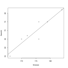
Graphic output of the example

A linear single regression can be carried out using the statistical software R. This can be done in R by the function lm , where the dependent variable is separated from the independent variables by the tilde. The summary function outputs the coefficients of the regression and other statistics:

# Lineare Regression mit Gewicht als Zielvariable
# Ergebnis wird als reg gespeichert:
reg <- lm(Gewicht~Groesse)

# Ausgabe der Ergebnisse der obigen linearen Regression:
summary(reg)

Diagrams are easy to create:

# Streudiagramm der Daten:
plot(Gewicht~Groesse)

# Regressionsgerade hinzufügen:
abline(reg)

Web links

Wikibooks: Introduction to Regression Calculation  - Learning and Teaching Materials

Commons : Linear Regression  - collection of images, videos and audio files

literature

• George G. Judge, R. Carter Hill, W. Griffiths, Helmut Lütkepohl , TC Lee. Introduction to the Theory and Practice of Econometrics. John Wiley & Sons, New York, Chichester, Brisbane, Toronto, Singapore, ISBN 978-0471624141 , second edition 1988.
• Norman R. Draper, Harry Smith: Applied Regression Analysis. Wiley, New York 1998.
• Ludwig von Auer : Econometrics. An introduction. Springer, ISBN 978-3-642-40209-8 , 6th through. u. updated edition 2013
• Ludwig Fahrmeir , Thomas Kneib , Stefan Lang, Brian Marx: Regression: models, methods and applications. Springer Science & Business Media, 2013, ISBN 978-3-642-34332-2
• Peter Schönfeld: Methods of Econometrics . Berlin / Frankfurt 1969.
• Dieter Urban, Jochen Mayerl: Regression analysis: theory, technology and application. 2., revised. Edition. VS Verlag, Wiesbaden 2006, ISBN 3-531-33739-4 .

Individual evidence

1. ^ W. Zucchini, A. Schlegel, O. Nenadíc, S. Sperlich: Statistics for Bachelor and Master students.
2. ^ ^{A b} Ludwig von Auer : Econometrics. An introduction. Springer, ISBN 978-3-642-40209-8 , 6th, through. u. updated edition. 2013, p. 49.
3. ↑ ^{a b} Jeffrey Marc Wooldridge : Introductory econometrics: A modern approach. 5th edition. Nelson Education 2015, p. 59.
4. ^ Karl Mosler and Friedrich Schmid: Probability calculation and conclusive statistics. Springer-Verlag, 2011, p. 292.
5. ↑ Jeffrey Marc Wooldridge: Introductory econometrics: A modern approach. 5th edition. Nelson Education 2015, p. 24.
6. ↑ ^{a b} Jeffrey Wooldridge: Introductory Econometrics: A Modern Approach . 5th international edition. South-Western, Mason, OH 2013, ISBN 978-1-111-53439-4 , pp. 113-114 (English).
7. ↑ JF Kenney, ES Keeping: Linear Regression and Correlation. In: Mathematics of Statistics. Pt. 1, 3rd edition. Van Nostrand, Princeton, NJ 1962, pp. 252-285.
8. ^ Rainer Schlittgen : Regression analyzes with R. 2013, ISBN 978-3-486-73967-1 , p. 4 (accessed via De Gruyter Online).
9. Analogous to ( argument of the maximum ), ↑ denotes the argument of the minimum ${\displaystyle \arg \min(\cdot )}$ ${\displaystyle \arg \max(\cdot )}$
10. ↑ Manfred Precht and Roland Kraft: Bio-Statistics 2: Hypothesis tests – analysis of variance – non-parametric statistics – analysis of contingency tables – correlation analysis – regression analysis – time series analysis – program examples in MINITAB, STATA, N, StatXact and TESTIMATE : 5., completely revised. Edition Reprint 2015, De Gruyter, Berlin June 2015, ISBN 978-3-486-78352-0 (accessed from De Gruyter Online), p. 299.
11. ^ Rainer Schlittgen: Regression analyzes with R. 2013, ISBN 978-3-486-73967-1 , p. 27 (accessed via De Gruyter Online).
12. ↑ Werner Timischl : Applied Statistics. An introduction for biologists and medical professionals. 2013, 3rd edition, p. 326.
13. ↑ Werner Timischl: Applied Statistics. An introduction for biologists and medical professionals. 2013, 3rd edition, p. 326.
14. ↑ George G. Judge, R. Carter Hill, W. Griffiths, Helmut Lütkepohl , TC Lee. Introduction to the Theory and Practice of Econometrics. 2nd Edition. John Wiley & Sons, New York / Chichester / Brisbane / Toronto / Singapore 1988, ISBN 0-471-62414-4 , p. 168.
15. ^ Ludwig Fahrmeir , Rita artist, Iris Pigeot , Gerhard Tutz : Statistics. The way to data analysis. 8., revised. and additional edition. Springer Spectrum, Berlin / Heidelberg 2016, ISBN 978-3-662-50371-3 , p. 443.
16. ↑ Jeffrey Marc Wooldridge: Introductory econometrics: A modern approach. 5th edition. Nelson Education 2015
17. ^ Karl Mosler and Friedrich Schmid: Probability calculation and conclusive statistics. Springer-Verlag, 2011, p. 308.
18. ↑ Werner Timischl : Applied Statistics. An introduction for biologists and medical professionals. 2013, 3rd edition, p. 313.
19. ^ Rainer Schlittgen: Regression analyzes with R. 2013, ISBN 978-3-486-73967-1 , p. 13 (accessed via De Gruyter Online).
20. ↑ Ludwig von Auer : Econometrics. An introduction. Springer, ISBN 978-3-642-40209-8 , 6th, through. u. updated edition. 2013, p. 135.
21. ^ Walter Gellert, Herbert Küstner, Manfred Hellwich, Herbert Kästner (Eds.): Small encyclopedia of mathematics. Leipzig 1970, pp. 669-670.
22. ↑ Jeffrey Marc Wooldridge: Introductory econometrics: A modern approach. 4th edition. Nelson Education, 2015, p. 57.
23. ↑ Lothar Sachs , Jürgen Hedderich: Applied Statistics: Collection of Methods with R. 8., revised. and additional edition. Springer Spectrum, Berlin / Heidelberg 2018, ISBN 978-3-662-56657-2 , p. 801