Constant equal distribution

Density function of the uniform distribution for (blue), (green) and (red) ${\displaystyle a=4,b=8}$ ${\displaystyle a=1,b=18}$ ${\displaystyle a=1,b=11}$

The constant uniform distribution , also called rectangular distribution , continuous uniform distribution , or uniform distribution , is a constant probability distribution . It has a constant probability density over an interval . This is synonymous with the fact that all sub-intervals of the same length have the same probability. ${\displaystyle [a,b]}$

The possibility of simulating the constant uniform distribution on the interval from 0 to 1 forms the basis for generating numerous randomly distributed random numbers using the inversion method or the rejection method .

definition

A continuous random variable is called uniformly distributed over the interval if the density function and distribution function are given as ${\displaystyle X}$ ${\displaystyle [a,b]}$ ${\displaystyle f(x)}$ ${\displaystyle F(x)}$

${\displaystyle f(x)={\begin{cases}{\frac {1}{b-a}}&a\leq x\leq b\\0&{\text{sonst.}}\end{cases}}={\frac {1}{\sqrt {12\sigma ^{2}}}}\cdot {\text{rect}}\left({\frac {x-\mu }{\sqrt {12\sigma ^{2}}}}\right)}$
${\displaystyle F(x)={\begin{cases}0&x\leq a\\{\frac {x-a}{b-a}}&a<x<b\\1&x\geq b\end{cases}}}$

Often or is used as an abbreviation for the constant uniform distribution . In some formulas one also sees or as a designation for the distribution. The constant uniform distribution is completely described by its first two central moments, i.e. H. all higher moments can be calculated from expected value and variance. ${\displaystyle {\mathcal {U}}(a,b)}$ ${\displaystyle {\mathcal {SG}}(a,b)}$ ${\displaystyle {\text{Gleich}}(a,b)}$ ${\displaystyle {\text{uniform}}(a,b)}$

properties

Probabilities

The probability that an evenly distributed random variable lies in a sub-interval is equal to the ratio of the interval lengths: ${\displaystyle [a,b]}$ ${\displaystyle X}$ ${\displaystyle [c,d]\subseteq [a,b]}$

${\displaystyle P(c\leq X\leq d)=F(d)-F(c)={\frac {d-c}{b-a}}}$.

Expected value and median

The expected value and the median of the constant uniform distribution are equal to the middle of the interval : ${\displaystyle [a,b]}$

${\displaystyle \operatorname {E} (X)=\int \limits _{-\infty }^{\infty }xf(x)\,dx={\frac {1}{b-a}}\int \limits _{a}^{b}x\cdot 1\,dx={\frac {1}{2}}{\frac {b^{2}-a^{2}}{b-a}}={\frac {a+b}{2}}}$

${\displaystyle \operatorname {Median} (X)=F^{-1}({\tfrac {1}{2}})={\frac {a+b}{2}}}$.

Variance

The variance of the constant uniform distribution is

${\displaystyle {\begin{aligned}\operatorname {Var} (X)&=\operatorname {E} (X^{2})-\left({\operatorname {E} (X)}\right)^{2}={\frac {1}{b-a}}\int \limits _{a}^{b}{x^{2}\cdot 1\,dx}-\left({\frac {a+b}{2}}\right)^{2}={\frac {1}{3}}{\frac {b^{3}-a^{3}}{b-a}}-\left({\frac {a+b}{2}}\right)^{2}\\&={\frac {1}{12}}\left({4b^{2}+4ab+4a^{2}-3a^{2}-6ab-3b^{2}}\right)={\frac {1}{12}}(b-a)^{2}.\end{aligned}}}$

Standard deviation and other measures of variance

The standard deviation is obtained from the variance

${\displaystyle \sigma (X)={\sqrt {\frac {(b-a)^{2}}{12}}}={\frac {b-a}{2{\sqrt {3}}}}\approx 0{,}289(b-a)}$.

The mean absolute deviation is , and the interquartile range is exactly twice as large. The uniform distribution is the only symmetrical distribution with monotonic density with this property. ${\displaystyle (b-a)/4}$ ${\displaystyle (b-a)/2}$

Coefficient of variation

The following results for the coefficient of variation :

${\displaystyle \operatorname {VarK} (X)={\frac {1}{\sqrt {3}}}{\frac {b-a}{a+b}}}$.

symmetry

The constant uniform distribution is symmetrical around . ${\displaystyle {\frac {a+b}{2}}}$

Crookedness

The skew can be represented as

${\displaystyle \operatorname {v} (X)=0}$.

Bulge and excess

The bulge and the excess can also be represented as closed ${\displaystyle \beta _{2}}$ ${\displaystyle \gamma _{2}=\beta _{2}-3}$

${\displaystyle \beta _{2}={\tfrac {9}{5}}=1{,}8}$ or.

${\displaystyle \gamma _{2}=-{\tfrac {6}{5}}=-1{,}2}$.

Moments

${\displaystyle k}$-th moment	${\displaystyle m_{k}={\frac {1}{k+1}}\sum _{i=0}^{k}a^{i}b^{k-i}={\frac {1}{k+1}}\sum _{i=0}^{k}\left(\mu -{\sqrt {3\sigma ^{2}}}\right)^{i}\left(\mu +{\sqrt {3\sigma ^{2}}}\right)^{k-i}}$
${\displaystyle k}$-th central moment	${\displaystyle \mu _{k}={\begin{cases}{\frac {(b-a)^{k}}{2^{k}(k+1)}}&{\text{ k gerade}}\\0&{\text{ k ungerade}}\end{cases}}={\begin{cases}{\frac {{\sqrt {3}}^{k}\sigma ^{k}}{(k+1)}}&{\text{ k gerade}}\\0&{\text{ k ungerade}}\end{cases}}}$

Sum of uniformly distributed random variables

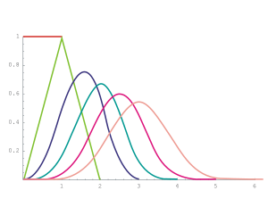
Distribution densities of the sum of up to 6 uniform distributions U (0.1)

The sum of two independent and continuously uniformly distributed random variables with the same carrier width is triangularly distributed , otherwise a trapezoidal distribution results. More accurate:

Let two random variables be independent and continuously evenly distributed, one on the interval , the other on the interval . Be and . Then their sum has the following trapezoidal distribution : ${\displaystyle [a,b]}$ ${\displaystyle [c,d]}$ ${\displaystyle \alpha =\min\{d-c,b-a\}}$ ${\displaystyle \beta =\max\{d-c,b-a\}}$

${\displaystyle f\colon \mathbb {R} \to \mathbb {R} ,x\longmapsto {\begin{cases}0&x\not \in [a+c,b+d]\\{\frac {x}{\alpha \beta }}-{\frac {a+c}{\alpha \beta }}&x\in [a+c,a+c+\alpha ]\\{\frac {1}{\beta }}&x\in [a+c+\alpha ,a+c+\beta ]\\{\frac {b+d}{\alpha \beta }}-{\frac {x}{\alpha \beta }}&x\in [a+c+\beta ,b+d]\end{cases}}}$

The sum of independent, uniformly distributed random variables on the interval [0; 1] is an Irwin-Hall distribution ; it approximates the normal distribution ( central limit theorem ).

An occasionally used method ( rule of twelve ) for the approximate generation of (standard) normally distributed random numbers works like this: one adds up 12 (independent) random numbers uniformly distributed over the interval [0,1] and subtracts 6 (this provides the correct moments, since the variance of a U (0,1) -distributed random variable is 1/12 and it has the expectation value 1/2).

Characteristic function

The characteristic function has the form

${\displaystyle \phi _{X}(t)={\frac {1}{(b-a)it}}\left(e^{itb}-e^{ita}\right)=\exp \left(i{\frac {b+a}{2}}t\right){\frac {\sin \left({\frac {b-a}{2}}t\right)}{{\frac {b-a}{2}}t}}}$,

where represents the imaginary unit . ${\displaystyle i}$

Moment generating function

The moment-generating function of the constant uniform distribution is

${\displaystyle m_{X}(s)={\begin{cases}{\frac {\displaystyle e^{bs}-e^{as}}{\displaystyle (b-a)s}}&s\neq 0\\1&s=0.\end{cases}}}$

and especially for and ${\displaystyle a=0}$ ${\displaystyle b=1}$

${\displaystyle m_{X}(s)={\frac {1}{s}}(e^{s}-1).}$

Relationship to other distributions

Relationship to the triangular distribution

The sum of two independent and continuously equally distributed random variables has a triangular distribution .

Relationship to beta distribution

If there are independent random variables that are constantly uniformly distributed, then the order statistics have a beta distribution . More precisely applies ${\displaystyle X_{1},X_{2},\dotsc ,X_{n}}$ ${\displaystyle [0,1]}$ ${\displaystyle X_{(1)},X_{(2)},\dotsc ,X_{(n)}}$

${\displaystyle X_{(k)}\sim B(k,n-k+1)}$

for . ${\displaystyle k=1,\dotsc ,n}$

Simulation of distributions from the constant uniform distribution

With the inversion method, uniformly distributed random numbers can be converted into other distributions. If is a uniformly distributed random variable, then, for example, the exponential distribution with the parameter is sufficient . ${\displaystyle X}$ ${\displaystyle Y=-{\tfrac {1}{\lambda }}\ln(X)}$ ${\displaystyle \lambda }$

Generalization to higher dimensions

The continuous uniform distribution can be from the interval in any measurable subsets of with Lebesgue measure generalize. Then you bet ${\displaystyle [a,b]}$ ${\displaystyle \Omega }$ ${\displaystyle \mathbb {R} ^{n}}$ ${\displaystyle 0<\lambda ^{n}(\Omega )<\infty }$

${\displaystyle {\mathcal {U}}_{\Omega }(A)=\int _{A}{\frac {1}{\lambda ^{n}(\Omega )}}\,dx={\frac {\lambda ^{n}(A)}{\lambda ^{n}(\Omega )}}}$

for measurable . ${\displaystyle A\subseteq \Omega }$

Discreet case

The uniform distribution is also defined on finite sets, then it is called discrete uniform distribution .

Example for the interval [0, 1]

Often it is and assumed, that is, considered. Then the density function on the interval is constant equal to 1 and the distribution function there applies . The expected value is accordingly , the variance and the standard deviation , whereby the latter two values ​​also apply to any intervals of length 1. See also the section above, Sum of uniformly distributed random variables . ${\displaystyle a=0}$ ${\displaystyle b=1}$ ${\displaystyle X\sim {\mathcal {U}}(0,1)}$ ${\displaystyle f}$ ${\displaystyle [0,1]}$ ${\displaystyle F(x)=x}$ ${\displaystyle E(X)={\tfrac {1}{2}}}$ ${\displaystyle \operatorname {Var} (X)={\tfrac {1}{12}}}$ ${\displaystyle \sigma (X)={\sqrt {\tfrac {1}{12}}}={\tfrac {1}{6}}{\sqrt {3}}\approx 0{,}29}$ ${\displaystyle [a,a+1]}$

Is a -distributed random variable, then is ${\displaystyle X}$ ${\displaystyle {\mathcal {U}}(0,1)}$

${\displaystyle Y=(b-a)X+a}$

${\displaystyle {\mathcal {U}}(a,b)}$-distributed.

See also

• Discrete equal distribution

literature

• Christian Hesse : Applied probability theory . 1st edition. Vieweg, Wiesbaden 2003, ISBN 3-528-03183-2 , pp. 155-156 , doi : 10.1007 / 978-3-663-01244-3 .

Web links

• Interactive animation - University of Konstanz