Negative binomial distribution

Negative binomial distribution
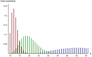
Probability distribution expected value = 10 orange; green the standard deviation
Distribution function
parameter	r > 0 - number of successes until termination p ∈ (0.1) - single success probability
carrier	k ∈ {0, 1, 2, 3,…} - number of failures
Probability function	${\displaystyle {k+r-1 \choose k}\cdot p^{r}(1-p)^{k}}$
Distribution function	${\displaystyle 1-I_{1-p}(k+1,\,r)}$ Euler's beta function
Expected value	${\displaystyle {\frac {r(1-p)}{p}}}$
mode	${\displaystyle \left\lfloor {\frac {(1-p)(r-1)}{p}}\right\rfloor }$
Variance	${\displaystyle {\frac {r(1-p)}{p^{2}}}}$
Crookedness	${\displaystyle {\frac {2-p}{\sqrt {r(1-p)}}}}$
Bulge	${\displaystyle {\frac {6}{r}}+{\frac {p^{2}}{r(1-p)}}}$
Moment generating function	${\displaystyle \left({\frac {pe^{s}}{1-(1-p)e^{s}}}\right)^{r}\!\!\!,s<|\ln(1-p)|}$
Characteristic function	${\displaystyle \left({\frac {pe^{\mathrm {i} s}}{1-(1-p)e^{\mathrm {i} s}}}\right)^{r}}$

The negative binomial distribution (also Pascal distribution ) is a univariate probability distribution . It is one of the discrete probability distributions and is one of the three Panjer distributions .

It describes the number of attempts that are required to achieve a given number of successes in a Bernoulli process .

In addition to the Poisson distribution , the negative binomial distribution is the most important loss number distribution in actuarial mathematics . There it is used in particular to distribute the number of claims in health insurance, less often in the area of ​​motor vehicle liability or comprehensive insurance.

Derivation of the negative binomial distribution

Probability function of the negative binomial distribution (variant A) for ; (blue), (green) and (red) ${\displaystyle r=10}$ ${\displaystyle p=0.2}$ ${\displaystyle p=0.5}$ ${\displaystyle p=0.8}$

This distribution can be described with the help of the urn model as putting back: In an urn there are two kinds of balls ( dichotomous population). The proportion of balls of the first kind is . The probability that a ball of first grade is pulled, thus amounts . ${\displaystyle p}$ ${\displaystyle p}$

A ball is drawn and put back again until the first type of balls is exactly of the first type. You can define a random variable : “Number of attempts to achieve success for the first time ”. The number of attempts depends on the amount . has a countably infinite number of possible manifestations. ${\displaystyle r}$ ${\displaystyle X}$ ${\displaystyle r}$ ${\displaystyle \{n\in \mathbb {N} |n\geq r\}}$ ${\displaystyle X}$

The probability that attempts were necessary to achieve success is calculated according to the following consideration: ${\displaystyle n}$ ${\displaystyle r}$ ${\displaystyle P(X=n)}$

Attempts are said to have already taken place at this point in time . A total of balls of the first kind were drawn. The probability of this is given by the binomial distribution of the random variables : "Number of balls of the first kind in experiments": ${\displaystyle n-1}$ ${\displaystyle r-1}$ ${\displaystyle Y}$ ${\displaystyle n-1}$

${\displaystyle \operatorname {P} (Y=r-1)={{n-1} \choose {r-1}}p^{r-1}(1-p)^{n-1-(r-1)}.}$

The probability that another ball of the first kind will be drawn is then

${\displaystyle \operatorname {P} (X=n)=\operatorname {P} (Y=r-1)\cdot p.}$

A random variable is called negative binomial distribution with the parameters (number of successful attempts) and (probability of occurrence of a success in an individual attempt) if the probability function applies to it ${\displaystyle X}$ ${\displaystyle \operatorname {NB} (r,p)}$ ${\displaystyle r}$ ${\displaystyle p}$

${\displaystyle \operatorname {P} (X=n)={{n-1} \choose {r-1}}p^{r}(1-p)^{n-r}}$

lets specify.

This variant is called variant A here to avoid confusion.

Alternative definition

A discrete random variable is subject to the negative binomial distribution with the parameters and , if they are the probabilities ${\displaystyle X}$ ${\displaystyle \operatorname {NB} (r,p)}$ ${\displaystyle r}$ ${\displaystyle p}$

${\displaystyle \operatorname {P} (X=k)={k+r-1 \choose k}p^{r}(1-p)^{k}={{k+r-1} \choose k}p^{r}q^{k}={{-r} \choose k}p^{r}(-q)^{k}}$

for owns. ${\displaystyle k=0,1,2\dotsc }$

Both definitions are related above ; While the first definition asks about the number of attempts (successful and unsuccessful) until the -th success occurs, the alternative representation is interested in the number of failures until the -th success occurs. The successes are not counted. The random variable then only describes the number of unsuccessful attempts. ${\displaystyle n=k+r}$ ${\displaystyle n}$ ${\displaystyle r}$ ${\displaystyle k}$ ${\displaystyle r}$ ${\displaystyle r}$ ${\displaystyle X}$

This variant is called variant B here .

Properties of the negative binomial distribution

Expected value

option A

The expected value is determined to be

${\displaystyle \operatorname {E} (X)={\frac {r}{p}}\,}$.

Variant B

With the alternative definition, the expected value is smaller, i.e. ${\displaystyle r}$

${\displaystyle \operatorname {E} (X)={\frac {r}{p}}-r={\frac {r(1-p)}{p}}}$.

Variance

The variance of the negative binomial distribution is given by for both definitions

${\displaystyle \operatorname {Var} (X)={\frac {r(1-p)}{p^{2}}}}$.

With the alternative definition, the variance is always greater than the expected value (over- dispersion ).

Coefficient of variation

option A

Of expectation and variance, the results immediately coefficient of variation to

${\displaystyle \operatorname {VarK} (X)={\sqrt {\frac {1-p}{r}}}}$

Variant B

In the alternative representation the result is

${\displaystyle \operatorname {VarK} (X)={\frac {1}{\sqrt {r(1-p)}}}}$.

Crookedness

The skew results for both variants as follows:

${\displaystyle \operatorname {v} (X)={\frac {2-p}{\sqrt {r(1-p)}}}}$.

Bulge

The excess is for both variants

${\displaystyle \gamma ={\frac {6}{r}}+{\frac {p^{2}}{r(1-p)}}}$.

So that is the bulge

${\displaystyle \beta _{2}={\frac {6}{r}}+{\frac {p^{2}}{r(1-p)}}+3}$.

Characteristic function

option A

The characteristic function has the form

${\displaystyle \varphi _{X}(s)=\left({\frac {pe^{\mathrm {i} s}}{1-(1-p)e^{\mathrm {i} s}}}\right)^{r}}$.

Variant B

Alternatively it arises

${\displaystyle \varphi _{X}(s)=\left({\frac {p}{1-(1-p)e^{is}}}\right)^{r}}$.

Probability generating function

option A

For the probability generating function one obtains

${\displaystyle m_{X}(s)=\left({\frac {ps}{1-(1-p)s}}\right)^{r}}$with . ${\displaystyle 0<s<{\frac {1}{1-p}}}$

Variant B

Analog is then

${\displaystyle m_{X}(s)=\left({\frac {p}{1-(1-p)s}}\right)^{r}}$.

Moment generating function

option A

The moment generating function of the negative binomial distribution is

${\displaystyle M_{X}(s)=\left({\frac {pe^{s}}{1-(1-p)e^{s}}}\right)^{r}}$with . ${\displaystyle s<|\ln(1-p)|}$

Variant B

Then there is the alternative display

${\displaystyle M_{X}(s)=\left({\frac {p}{1-(1-p)e^{s}}}\right)^{r}}$

Sums of negative binomial random variables

Are two independent negative binomial random variables for the parameters and . Then there is again a negative binomial distribution for the parameter and . The negative binomial distribution is thus reproductively , for folding applies , ${\displaystyle X_{1},X_{2}}$ ${\displaystyle r_{1},r_{2}}$ ${\displaystyle p}$ ${\displaystyle X_{1}+X_{2}}$ ${\displaystyle r_{1}+r_{2}}$ ${\displaystyle p}$ ${\displaystyle \operatorname {NB} (r_{1},p)*\operatorname {NB} (r_{2},p)=\operatorname {NB} (r_{1}+r_{2},p)}$

it forms a folding semi-group .

Generalization to real parameters

The above derivation and interpretation of the negative binomial distribution using the urn model is only possible for. However, there is also a generalization of the negative binomial distribution for . For this purpose, a Poisson distribution is considered, the intensity of which is randomly distributed according to a gamma distribution with the parameters and . If the mixed distribution of these two distributions is now formed, the so-called Poisson-gamma distribution results . The following then applies to the probability function of this distribution ${\displaystyle r\in \mathbb {N} }$ ${\displaystyle r\in \mathbb {R} ^{+}}$ ${\displaystyle P(k|\lambda )}$ ${\displaystyle \lambda }$ ${\displaystyle r}$ ${\displaystyle {\frac {p}{1-p}}}$

${\displaystyle {\begin{aligned}f(k|r,p)&=\int _{0}^{\infty }f_{\text{Poi}}(k|\lambda )\cdot f_{\text{Gamma}}(\lambda |r,{\frac {p}{1-p}})\;\mathrm {d} \lambda \\[8pt]&=\int _{0}^{\infty }{\frac {\lambda ^{k}}{k!}}e^{-\lambda }\cdot \lambda ^{r-1}{\frac {e^{-\lambda p/(1-p)}}{{\big (}{\frac {1-p}{p}}{\big )}^{r}\,\Gamma (r)}}\;\mathrm {d} \lambda \\[8pt]&={\frac {p^{r}(1-p)^{-r}}{k!\,\Gamma (r)}}\int _{0}^{\infty }\lambda ^{r+k-1}e^{-\lambda /(1-p)}\;\mathrm {d} \lambda \\[8pt]&={\frac {(p)^{r}(1-p)^{-r}}{k!\,\Gamma (r)}}\ (1-p)^{r+k}\,\Gamma (r+k)\\[8pt]&={\frac {\Gamma (r+k)}{k!\;\Gamma (r)}}\;(1-p)^{k}p^{r}.\end{aligned}}}$

For is the probability function of the negative binomial distribution. Thus, the negative binomial distribution can also be interpreted as meaningful. The probability of achieving success is then equal to the probability of achieving success with a binomial distribution with random, gamma-distributed parameters . The gamma functions in the probability function can also be replaced by generalized binomial coefficients. ${\displaystyle r\in \mathbb {N} }$ ${\displaystyle r\in \mathbb {R} ^{+}}$ ${\displaystyle k}$ ${\displaystyle k}$

This construction corresponds to variant B defined above. All characteristics, such as expected value, variance and so on, remain unchanged. In addition, the variant for real is infinitely divisible . ${\displaystyle r>0}$

Relationships with other distributions

Relationship to the geometric distribution

The negative binomial distribution goes over into the geometric distribution . On the other hand, the sum of mutually independent geometrically distributed random variables with the same parameter is negative-binomially distributed with the parameters and . However, it should also be noted here which parameterization variant was selected. ${\displaystyle r=1}$ ${\displaystyle X=\sum _{i=1}^{r}X_{i}}$ ${\displaystyle X_{1},\dots ,X_{r}}$ ${\displaystyle p}$ ${\displaystyle \operatorname {NB} (r,p)}$ ${\displaystyle p}$ ${\displaystyle r}$

Relationship to the composite Poisson distribution

The negative binomial distribution arises from the composite Poisson distribution when combined with the logarithmic distribution . The parameters go to variant B with and . ${\displaystyle p_{\text{log}}=1-p_{\text{neg}}}$ ${\displaystyle \textstyle r={\frac {-\lambda }{\ln(1-p_{\text{log}})}}}$

example

Probability function of the negative binomial distribution

Distribution function of the negative binomial distribution

The student Paula is playing skat tonight. She knows from long experience that she wins every fifth game. Winning is defined as follows: you must first get a game by bidding, then you have to win this game.

Since she has a statistics lecture at eight o'clock tomorrow, the evening shouldn't be too long. That's why she decided to go home after winning the 10th game. Let us assume that a game lasts about 4 minutes (generously calculated). What is the probability that she can go home after two hours, that is, after 30 games?

We proceed with our considerations in the same way as above:

What is the probability that she won 9 times in 29 games? We calculate this probability with the binomial distribution, in terms of the urn model with 29 attempts and 9 balls of the first sort:

${\displaystyle P(Y=9)={29 \choose 9}0{,}2^{9}\cdot 0{,}8^{20}=0{,}0591.}$

The probability of making the 10th win on the 30th game is now

${\displaystyle P(X=30)=0{,}0591\cdot 0{,}2=0{,}0118.}$

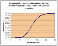
This probability now seems to be very small. The graph of the negative binomial random variable X shows that overall the probabilities remain very small. How is poor Paula ever supposed to get to bed? We can reassure her: it is enough to ask how many attempts Paula needs at most , it doesn't have to be exactly 30.

The probability that a maximum of 30 attempts are necessary is the distribution function F (x) of the negative binomial distribution at x = 30, which here is the sum of the probabilities P (X = 0) + P (X = 1) + P (X = 2) + ... + P (X = 30) results. A look at the graph of the distribution function shows: If Paula is satisfied with a 50% probability, she would have to play at most about 50 games, that would be 50 · 4 min = 200 min = 3h 20 min. In order to get her 10 winnings with an 80% probability, she would have to play a maximum of about 70 games, i.e. almost 5 hours. Maybe Paula should change her game number strategy after all.

Web links

• AV Prokhorov: Negative binomial distribution . In: Michiel Hazewinkel (Ed.): Encyclopaedia of Mathematics . Springer-Verlag , Berlin 2002, ISBN 978-1-55608-010-4 (English, online ).
• Eric W. Weisstein : Negative Binomial Distribution . In: MathWorld (English).

literature

• Achim Klenke: Probability Theory . 3. Edition. Springer-Verlag, Berlin Heidelberg 2013, ISBN 978-3-642-36017-6 , doi : 10.1007 / 978-3-642-36018-3 .
• Christian Hesse: Applied probability theory . 1st edition. Vieweg, Wiesbaden 2003, ISBN 3-528-03183-2 , doi : 10.1007 / 978-3-663-01244-3 .