Multiple linear regression

In statistics , multiple linear regression , also known as multiple linear regression ( MLR for short ) or linear multiple regression , is a regression analysis method and a special case of linear regression . Multiple linear regression is a statistical technique that attempts to explain an observed dependent variable in terms of several independent variables . The model used for this is linear in the parameters, with the dependent variable being a function of the independent variables. This relationship is overlaid by an additive disturbance variable . The multiple linear regression represents a generalization of the simple linear regression with regard to the number of regressors.

The classic model of linear multiple regression

Play media file

Regression plane that adapts to a "point cloud" in three-dimensional space (case ) ${\displaystyle K=3}$

In the following, linear functions are assumed. It is then no further restriction of generality that these functions consist directly of the independent (explanatory, exogenous) variables and that there are as many regression parameters to be estimated as there are independent variables (index ). For comparison: In simple linear regression, and is constant , the associated regression parameter is the axis intercept . ${\displaystyle \beta _{k}}$ ${\displaystyle x_{k}}$ ${\displaystyle k=1,2,\dots ,K}$ ${\displaystyle K=2}$ ${\displaystyle x_{1}}$ ${\displaystyle 1}$

The model for measurements of the dependent (endogenous) variables is ${\displaystyle T}$ ${\displaystyle y}$

${\displaystyle y_{t}=x_{t1}\beta _{1}+x_{t2}\beta _{2}+\ldots +x_{tK}\beta _{K}+\varepsilon _{t}}$,

with disturbances that are purely random if the linear model fits. For the model, it is further assumed that the Gauss-Markov assumptions apply. In a sample theoretical approach, each sample element is interpreted as a separate random variable , as is each one . ${\displaystyle \varepsilon _{t}}$ ${\displaystyle \varepsilon _{t}}$ ${\displaystyle y_{t}}$

Are the data

${\displaystyle (y_{1};x_{11},\dotsc ,x_{1K}),(y_{2};x_{21},\dotsc ,x_{2K}),\dotsc ,(y_{T};x_{T1},\dotsc ,x_{TK})}$

then the following system of linear equations results :

${\displaystyle {\begin{matrix}y_{1}=x_{11}\beta _{1}+x_{12}\beta _{2}\,+&\dotsb &+\,x_{1K}\beta _{K}+\varepsilon _{1}\\y_{2}=x_{21}\beta _{1}+x_{22}\beta _{2}\,+&\dotsb &+\,x_{2K}\beta _{K}+\varepsilon _{2}\\&\vdots &\\y_{T}=x_{T1}\beta _{1}+x_{T2}\beta _{2}\,+&\dotsb &+\,x_{TK}\beta _{K}+\varepsilon _{T}\\\end{matrix}}}$

The multiple linear regression model (rare and ambiguous general linear model) can be formulated in matrix notation as follows

${\displaystyle \mathbf {y} =\mathbf {X} {\boldsymbol {\beta }}+{\boldsymbol {\varepsilon }}}$.

This is the underlying model in the population  and is also known as the “ true model ”. Here stand , and for the vectors or matrices: ${\displaystyle \mathbf {y} }$ ${\displaystyle {\boldsymbol {\varepsilon }}}$ ${\displaystyle {\boldsymbol {\beta }}}$

${\displaystyle \mathbf {y} ={\begin{pmatrix}y_{1}\\y_{2}\\\vdots \\y_{t}\\\vdots \\y_{T}\end{pmatrix}}_{(T\times 1)}\;,\;\;\;\;\;}$ ${\displaystyle {\boldsymbol {\varepsilon }}={\begin{pmatrix}\varepsilon _{1}\\\varepsilon _{2}\\\vdots \\\varepsilon _{t}\\\vdots \\\varepsilon _{T}\end{pmatrix}}_{(T\times 1)}\;\;\;\;}$ and ${\displaystyle \;\;\;{\boldsymbol {\beta }}={\begin{pmatrix}\beta _{1}\\\beta _{2}\\\vdots \\\beta _{k}\\\vdots \\\beta _{K}\end{pmatrix}}_{(K\times 1)}}$

and a matrix (test plan or data matrix ): ${\displaystyle \mathbf {X} }$ ${\displaystyle T\times K}$

${\displaystyle \mathbf {X} ={\begin{pmatrix}x_{11}&x_{12}&\cdots &x_{1k}&\cdots &x_{1K}\\x_{21}&x_{22}&\cdots &x_{2k}&\cdots &x_{2K}\\\vdots &\vdots &\ddots &\vdots &\ddots &\vdots \\x_{t1}&x_{t2}&\cdots &x_{tk}&\cdots &x_{tK}\\\vdots &\vdots &\ddots &\vdots &\ddots &\vdots \\x_{T1}&x_{T2}&\cdots &x_{Tk}&\cdots &x_{TK}\end{pmatrix}}_{(T\times K)}={\begin{pmatrix}\ \mathbf {x} _{1}^{\top }\\\ \mathbf {x} _{2}^{\top }\\\vdots \\\ \mathbf {x} _{t}^{\top }\\\vdots \\\\\mathbf {x} _{T}^{\top }\end{pmatrix}}_{(T\times K)}={\begin{pmatrix}\mathbf {x} _{(1)}\mathbf {x} _{(2)}&\cdots &\mathbf {x} _{(k)}&\cdots &\mathbf {x} _{(K)}\end{pmatrix}}_{(T\times K)}\quad }$, in which ${\displaystyle \quad \mathbf {x} _{(1)}\equiv 1\!\!1_{T}={\begin{pmatrix}1\\1\\\vdots \\1\\\vdots \\1\end{pmatrix}}_{(T\times 1)}}$

Due to the different spellings for , it can be seen that the model can also be represented as: ${\displaystyle \mathbf {X} }$ ${\displaystyle \mathbf {y} =\mathbf {X} {\boldsymbol {\beta }}+{\boldsymbol {\varepsilon }}}$

${\displaystyle y_{t}=x_{t1}\beta _{1}+x_{t2}\beta _{2}+\dotsb +x_{tK}\beta _{K}+\varepsilon _{t}=\mathbf {x} _{t}^{\top }{\boldsymbol {\beta }}+\varepsilon _{t},\quad t=1,2,\dotsc ,T}$

With

${\displaystyle \mathbf {x} _{t}={\begin{pmatrix}\ x_{t1}\\\ x_{t2}\\\vdots \\\ x_{tk}\\\vdots \\\\x_{tK}\end{pmatrix}}_{(K\times 1)}}$,

where is the observed dependent variable for observation and , are the independent variables. As usual, the absolute term and are unknown scalar slope parameters. The disturbance for observation is an unobservable random variable. The vector is the transposed vector of the regressors and is also known as the linear predictor  . ${\displaystyle y_{t}}$ ${\displaystyle t}$ ${\displaystyle x_{tk}\;,t=1,\ldots ,T}$ ${\displaystyle \beta _{1}}$ ${\displaystyle \beta _{2},\beta _{3},\dotsc ,\beta _{K}}$ ${\displaystyle \varepsilon _{t}}$ ${\displaystyle t}$ ${\displaystyle \mathbf {x} _{t}^{\top }}$ ${\displaystyle \mathbf {x} _{t}^{\top }{\boldsymbol {\beta }}}$

The essential prerequisite for the multiple linear regression model is that it describes the “ true model ” apart from the disturbance variable . As a rule, it is not specified exactly what type of disturbance variable is; for example, it can result from additional factors or measurement errors. However, one assumes as a basic requirement that its expected value (in all components) is 0: (assumption 1). This assumption means that the model is generally considered to be correct and the observed deviation is regarded as random or originates from negligible external influences. Typical is the assumption that the components of the vector uncorrelated are (Assumption 2) and the same variance own (Assumption 3), thereby using classical methods such as the method of least squares ( english ordinary least squares , in short: OLS ) simple estimator the unknown parameters and result. The method is therefore (multiple linear) least squares regression ( English OLS regression called). ${\displaystyle {\boldsymbol {\varepsilon }}}$ ${\displaystyle \operatorname {E} ({\boldsymbol {\varepsilon }})={\boldsymbol {0}}}$ ${\displaystyle \sigma ^{2}}$ ${\displaystyle {\boldsymbol {\beta }}}$ ${\displaystyle \sigma ^{2}}$

In summary, it is assumed for the disturbance variables that

• (A1) have zero expected value: , ${\displaystyle \operatorname {E} ({\boldsymbol {\varepsilon }})=\mathbf {0} \ }$
• (A2) are uncorrelated: and ${\displaystyle \operatorname {Cov} (\varepsilon _{t},\varepsilon _{s})=\operatorname {E} [(\varepsilon _{t}-\operatorname {E} (\varepsilon _{t}))((\varepsilon _{s}-\operatorname {E} (\varepsilon _{s}))]=\operatorname {E} (\varepsilon _{t}\varepsilon _{s})=0\quad \forall t\neq s}$
• (A3) have a homogeneous variance : (scalar covariance matrix). ${\displaystyle {\mbox{Cov}}({\boldsymbol {\varepsilon }})=\sigma ^{2}\mathbf {I} _{T}}$

Here denotes the zero vector and the unit matrix of the dimension . The above assumptions are the assumptions of classical linear regression . The model (the equation together with the above assumptions) is therefore called the classical model of linear multiple regression . ${\displaystyle \mathbf {0} }$ ${\displaystyle \mathbf {I} _{T}}$ ${\displaystyle T}$ ${\displaystyle \mathbf {y} =\mathbf {X} {\boldsymbol {\beta }}+{\boldsymbol {\varepsilon }}}$

Instead of just looking at the variances and covariances of the disturbance variables individually, they are summarized in the following covariance matrix :

${\displaystyle {\begin{aligned}{\mbox{Cov}}({\boldsymbol {\varepsilon }})&=\operatorname {E} \left(({\boldsymbol {\varepsilon }}-\underbrace {\operatorname {E} ({\boldsymbol {\varepsilon }})} _{=\mathbf {0} \;{\text{aus A1}}})({\boldsymbol {\varepsilon }}-\underbrace {\operatorname {E} ({\boldsymbol {\varepsilon }})} _{=\mathbf {0} \;{\text{aus A1}}})^{\top }\right)=\operatorname {E} ({\boldsymbol {\varepsilon }}{\boldsymbol {\varepsilon }}^{\top })={\begin{pmatrix}\operatorname {Var} (\varepsilon _{1})&\operatorname {Cov} (\varepsilon _{1},\varepsilon _{2})&\cdots &\operatorname {Cov} (\varepsilon _{1},\varepsilon _{T})\\\\\operatorname {Cov} (\varepsilon _{2},\varepsilon _{1})&\operatorname {Var} (\varepsilon _{2})&\cdots &\operatorname {Cov} (\varepsilon _{2},\varepsilon _{T})\\\\\vdots &\vdots &\ddots &\vdots \\\\\operatorname {Cov} (\varepsilon _{T},\varepsilon _{1})&\operatorname {Cov} (\varepsilon _{T},\varepsilon _{2})&\cdots &\operatorname {Var} (\varepsilon _{T})\end{pmatrix}}\\&{\stackrel {\text{aus A2}}{=}}{\begin{pmatrix}\sigma ^{2}&0&\cdots &0\\0&\sigma ^{2}&\ddots &\vdots \\\vdots &\ddots &\ddots &0\\0&\cdots &0&\sigma ^{2}\end{pmatrix}}_{(T\times T)}=\sigma ^{2}\mathbf {I} _{T}\end{aligned}}}$

Thus for ${\displaystyle \mathbf {y} }$

${\displaystyle \operatorname {E} (\mathbf {y} )=\mathbf {X} {\boldsymbol {\beta }}\quad }$with . ${\displaystyle \quad {\mbox{Cov}}(\mathbf {y} )={\mbox{Cov}}({\boldsymbol {\varepsilon }})=\sigma ^{2}\mathbf {I} _{T}}$

Beyond this basic assumption, all distribution assumptions an are generally permitted. If it is also assumed that the vector is multidimensionally normally distributed , it can also be shown that the two estimators are solutions of the maximum likelihood equations (see #Statistical Inference ). In this model, the independence of the disturbance variables is then equivalent to that of the . ${\displaystyle {\boldsymbol {\varepsilon }}}$ ${\displaystyle {\boldsymbol {\varepsilon }}}$ ${\displaystyle y_{t}}$

Estimation of the parameter vector with least squares estimation

In the multiple linear regression model, too, the vector of the disturbance variables is minimized with the help of least squares estimation (KQ estimation), that is, it should be chosen so that the Euclidean norm is minimal. In the following, the approach is used that the residual sum of squares is minimized. This assumes that has the rank . Then it is invertible and one obtains as a minimization problem : ${\displaystyle {\boldsymbol {\beta }}}$ ${\displaystyle \|\mathbf {y} -\mathbf {X} {\boldsymbol {\beta }}\|_{2}}$ ${\displaystyle \mathbf {X} }$ ${\displaystyle K}$ ${\displaystyle \mathbf {X} ^{\top }\mathbf {X} }$

${\displaystyle {\underset {\boldsymbol {\beta }}{\rm {arg\,min}}}\,Q({\boldsymbol {\beta }})={\underset {\boldsymbol {\beta }}{\rm {arg\,min}}}\,(\mathbf {y} -\mathbf {X} {\boldsymbol {\beta }})^{\top }(\mathbf {y} -\mathbf {X} {\boldsymbol {\beta }})={\underset {\boldsymbol {\beta }}{\rm {arg\,min}}}\,\sum _{t=1}^{T}(y_{t}-\mathbf {x} _{t}^{\top }{\boldsymbol {\beta }})^{2}={\underset {\boldsymbol {\beta }}{\rm {arg\,min}}}\,\left(\mathbf {y} ^{\top }\mathbf {y} -2{\boldsymbol {\beta }}^{\top }\mathbf {X} ^{\top }\mathbf {y} +{\boldsymbol {\beta }}^{\top }\mathbf {X} ^{\top }\mathbf {X} {\boldsymbol {\beta }}\right)}$

The first order condition (zeroing the gradient ) is:

${\displaystyle {\frac {\partial \,Q({\boldsymbol {\beta }})}{\partial {\boldsymbol {\beta }}}}={\begin{pmatrix}{\frac {\partial \,Q({\boldsymbol {\beta }})}{\partial \beta _{1}}}\\{\frac {\partial \,Q({\boldsymbol {\beta }})}{\partial \beta _{2}}}\\\vdots \\{\frac {\partial \,Q({\boldsymbol {\beta }})}{\partial \beta _{K}}}\end{pmatrix}}{\overset {\mathrm {!} }{=}}\;\mathbf {0} }$

The least squares estimate can be interpreted as a projection onto the plane spanned by the regressors.

The first order partial derivatives are:

${\displaystyle {\begin{aligned}{\frac {\partial \,Q({\boldsymbol {\beta }})}{\partial \beta _{1}}}&={\frac {\partial (\mathbf {y} ^{\top }\mathbf {y} )}{\partial \beta _{1}}}-{\frac {\partial (2{\boldsymbol {\beta }}^{\top }\mathbf {X} ^{\top }\mathbf {y} )}{\partial \beta _{1}}}+{\frac {\partial ({\boldsymbol {\beta }}^{\top }\mathbf {X} ^{\top }\mathbf {X} {\boldsymbol {\beta }})}{\partial \beta _{1}}}=-2\mathbf {x} _{(1)}^{\top }\mathbf {y} +2\mathbf {x} _{(1)}^{\top }\mathbf {X} {\boldsymbol {\beta }}\\{\frac {\partial \,Q({\boldsymbol {\beta }})}{\partial \beta _{2}}}&={\frac {\partial (\mathbf {y} ^{\top }\mathbf {y} )}{\partial \beta _{2}}}-{\frac {\partial (2{\boldsymbol {\beta }}^{\top }\mathbf {X} ^{\top }\mathbf {y} )}{\partial \beta _{2}}}+{\frac {\partial ({\boldsymbol {\beta }}^{\top }\mathbf {X} ^{\top }\mathbf {X} {\boldsymbol {\beta }})}{\partial \beta _{2}}}=-2\mathbf {x} _{(2)}^{\top }\mathbf {y} +2\mathbf {x} _{(2)}^{\top }\mathbf {X} {\boldsymbol {\beta }}\\\vdots \\{\frac {\partial \,Q({\boldsymbol {\beta }})}{\partial \beta _{K}}}&={\frac {\partial (\mathbf {y} ^{\top }\mathbf {y} )}{\partial \beta _{K}}}-{\frac {\partial (2{\boldsymbol {\beta }}^{\top }\mathbf {X} ^{\top }\mathbf {y} )}{\partial \beta _{K}}}+{\frac {\partial ({\boldsymbol {\beta }}^{\top }\mathbf {X} ^{\top }\mathbf {X} {\boldsymbol {\beta }})}{\partial \beta _{K}}}=-2\mathbf {x} _{(K)}^{\top }\mathbf {y} +2\mathbf {x} _{(K)}^{\top }\mathbf {X} {\boldsymbol {\beta }}\end{aligned}}}$

This shows that the first order condition for the vector of the estimated regression parameters can be compactly represented as: ${\displaystyle \mathbf {b} }$

${\displaystyle \left.{\frac {\partial Q({\boldsymbol {\beta }})}{\partial \mathbf {\beta } }}\right|_{\mathbf {b} }=-2\mathbf {X} ^{\top }\mathbf {y} +2\mathbf {X} ^{\top }\mathbf {X} \mathbf {b} \;{\overset {\mathrm {!} }{=}}\;\mathbf {0} }$

or.

${\displaystyle \mathbf {X} ^{\top }\mathbf {X} \mathbf {b} =\mathbf {X} ^{\top }\mathbf {y} }$.

This system of linear equations is usually called the (Gaussian) normal equation system .

Since the matrix to rank does that is square symmetric matrix non-singular and the inverse for exists. Therefore, after multiplying on the left with the inverse of the product sum matrix, the following vector of the estimated regression coefficients is obtained as a solution to the minimization problem: ${\displaystyle \mathbf {X} }$ ${\displaystyle K}$ ${\displaystyle \mathbf {X} ^{\top }\mathbf {X} }$ ${\displaystyle \mathbf {X} ^{\top }\mathbf {X} }$ ${\displaystyle (\mathbf {X} ^{\top }\mathbf {X} )^{-1}}$

${\displaystyle \mathbf {b} ={\begin{pmatrix}b_{1}\\b_{2}\\b_{2}\\\vdots \\b_{K}\end{pmatrix}}=(\mathbf {X} ^{\top }\mathbf {X} )^{-1}\mathbf {X} ^{\top }\mathbf {y} }$

If the rank is less than , then it is not invertible, i.e. the system of normal equations cannot be uniquely solved, and therefore not identifiable , but see the concept of estimability . Since the residual sum of squares is minimized, it is also called a least squares estimator (short: KQ estimator). Alternatively, the least squares estimator can also be represented as, using the true model ${\displaystyle \mathbf {X} }$ ${\displaystyle K}$ ${\displaystyle \mathbf {X} ^{\top }\mathbf {X} }$ ${\displaystyle \mathbf {b} }$ ${\displaystyle \mathbf {b} }$ ${\displaystyle \mathbf {b} }$ ${\displaystyle \mathbf {y} =\mathbf {X} {\boldsymbol {\beta }}+{\boldsymbol {\varepsilon }}}$

${\displaystyle \mathbf {b} =(\mathbf {X} ^{\top }\mathbf {X} )^{-1}\mathbf {X} ^{\top }(\mathbf {X} {\boldsymbol {\beta }}+{\boldsymbol {\varepsilon }})={\boldsymbol {\beta }}+(\mathbf {X} ^{\top }\mathbf {X} )^{-1}\mathbf {X} ^{\top }{\boldsymbol {\varepsilon }}}$

For the covariance matrix of the least squares estimator we get (shown in compact form):

${\displaystyle \operatorname {Cov} (\mathbf {b} )={\boldsymbol {\beta }}+(\mathbf {X} ^{\top }\mathbf {X} )^{-1}\mathbf {X} ^{\top }{\boldsymbol {\varepsilon }}=(\mathbf {X} ^{\top }\mathbf {X} )^{-1}\mathbf {X} ^{\top }\operatorname {Cov} (\mathbf {Y} )\ \mathbf {X} (\mathbf {X} ^{\top }\mathbf {X} )^{-1}=\sigma ^{2}(\mathbf {X} ^{\top }\mathbf {X} )^{-1}=\Sigma _{\mathbf {b} }}$

In the case of linear single regression ( ), the above formula is reduced to the known expressions for the variances of the LQ estimators and (see Statistical Properties of Least Squares Estimators ). ${\displaystyle {\boldsymbol {\beta }}=(\beta _{1},\beta _{2})^{\top }}$ ${\displaystyle \operatorname {Var} (\beta _{2})={\frac {\sigma ^{2}}{\sum _{t=1}^{T}(x_{t2}-{\overline {x}}_{2})^{2}}}}$ ${\displaystyle \operatorname {Var} (\beta _{1})={\frac {\sigma ^{2}\sum _{t=1}^{T}x_{t2}^{2}}{T\sum _{t=1}^{T}(x_{t2}-{\overline {x}}_{2})^{2}}}}$

proof

${\displaystyle {\begin{aligned}\sigma ^{2}(\mathbf {X} ^{\top }\mathbf {X} )^{-1}&=\sigma ^{2}\left({\begin{pmatrix}1&1&\cdots \\x_{12}&x_{22}&\cdots \end{pmatrix}}{\begin{pmatrix}1&x_{12}\\1&x_{22}\\\vdots &\vdots \,\,\,\end{pmatrix}}\right)^{-1}\\[6pt]&=\sigma ^{2}\left(\sum _{t=1}^{T}{\begin{pmatrix}1&x_{t2}\\x_{t2}&x_{t2}^{2}\end{pmatrix}}\right)^{-1}\\[6pt]&=\sigma ^{2}{\begin{pmatrix}T&\sum x_{t2}\\\sum x_{t2}&\sum x_{t2}^{2}\end{pmatrix}}^{-1}\\[6pt]&=\sigma ^{2}\cdot {\frac {1}{T\sum x_{t2}^{2}-(\sum x_{i2})^{2}}}{\begin{pmatrix}\sum x_{t2}^{2}&-\sum x_{t2}\\-\sum x_{t2}&T\end{pmatrix}}\\[6pt]&=\sigma ^{2}\cdot {\frac {1}{T\sum {(x_{t2}-{\overline {x}})^{2}}}}{\begin{pmatrix}\sum x_{t2}^{2}&-\sum x_{t2}\\-\sum x_{t2}&T\end{pmatrix}}\\[8pt]\Rightarrow \operatorname {Var} (\beta _{1})&=\sigma ^{2}(\mathbf {X} ^{\top }\mathbf {X} )_{11}^{-1}={\frac {\sigma ^{2}\sum _{t=1}^{T}x_{t2}^{2}}{T\sum _{t=1}^{T}(x_{t2}-{\overline {x}}_{2})^{2}}}\\\Rightarrow \operatorname {Var} (\beta _{2})&=\sigma ^{2}(\mathbf {X} ^{\top }\mathbf {X} )_{22}^{-1}={\frac {\sigma ^{2}}{\sum _{t=1}^{T}(x_{t2}-{\overline {x}}_{2})^{2}}}.\end{aligned}}}$

Using the least squares estimator is obtained the equation system ${\displaystyle \mathbf {b} }$

${\displaystyle {\hat {\mathbf {y} }}=\mathbf {X} \mathbf {b} =\mathbf {y} -{\hat {\boldsymbol {\varepsilon }}}}$,

where is the vector of residuals and the estimate is for . The interest of analysis often lies in estimating or predicting the dependent variable for a given tuple of . The prediction vector is calculated as ${\displaystyle {\hat {\boldsymbol {\varepsilon }}}}$ ${\displaystyle {\hat {\mathbf {y} }}}$ ${\displaystyle \mathbf {y} }$ ${\displaystyle {\hat {\mathbf {y} }}_{0}}$ ${\displaystyle \mathbf {y} }$ ${\displaystyle {\mathbf {x} }_{0}}$

${\displaystyle {\hat {\mathbf {y} }}_{0}=x_{01}b_{1}+x_{02}b_{2}+\dotsc +x_{0K}b_{K}=\mathbf {x} _{0}^{\top }{\mathbf {b} }}$.

Quality properties of the least squares estimator

Expectancy

In the multiple case, just as in the simple case, one can show that the least squares estimation vector is unbiased for . However, this only applies if the assumption that the regressors are exogenous is given. This is the case when the possibly random regressors and the disturbance variables are uncorrelated, i.e. H. if applies. If one assumes here that the exogenous variables are not random variables, but can be controlled as in an experiment , then applies or and is therefore true to expectation for . ${\displaystyle {\boldsymbol {\beta }}}$ ${\displaystyle \operatorname {E} (\mathbf {x} ^{\top }\mathbf {\cdot } {\boldsymbol {\varepsilon }})\mathbf {=} 0}$ ${\displaystyle \forall k\in \{1,\dotsc ,K\}\colon \operatorname {E} (x_{tk}\varepsilon _{t})=x_{tk}\cdot \operatorname {E} (\varepsilon _{t})=0}$ ${\displaystyle \operatorname {E} (\mathbf {x} ^{\top }\mathbf {\cdot } {\boldsymbol {\varepsilon }})=\mathbf {0} }$ ${\displaystyle \mathbf {b} }$ ${\displaystyle {\boldsymbol {\beta }}}$

proof

${\displaystyle {\begin{aligned}\operatorname {E} (\mathbf {b} )&=\operatorname {E} ((\mathbf {X} ^{\top }\mathbf {X} )^{-1}\mathbf {X} ^{\top }\mathbf {y} )\\&=\operatorname {E} ((\mathbf {X} ^{\top }\mathbf {X} )^{-1}\mathbf {X} ^{\top }(\mathbf {X} {\boldsymbol {\beta }}+{\boldsymbol {\varepsilon }}))\\&=\operatorname {E} ((\mathbf {X} ^{\top }\mathbf {X} )^{-1}\mathbf {X} ^{\top }\mathbf {X} {\boldsymbol {\beta }}+(\mathbf {X} ^{\top }\mathbf {X} )^{-1}\mathbf {X} ^{\top }{\boldsymbol {\varepsilon }}))=(\mathbf {X} ^{\top }\mathbf {X} )^{-1}(\mathbf {X} ^{\top }\mathbf {X} ){\boldsymbol {\beta }}+(\mathbf {X} ^{\top }\mathbf {X} )^{-1}\underbrace {\operatorname {E} (\mathbf {X} ^{\top }{\boldsymbol {\varepsilon }})} _{=\mathbf {0} }={\boldsymbol {\beta }}\end{aligned}}}$

If the assumption of exogeneity does not apply, the least squares estimator is not fair to expectations for . So there is a distortion ( English bias ), i. In other words, "on average" the parameter estimate deviates from the true parameter: ${\displaystyle \operatorname {E} (\mathbf {x} ^{\top }{\boldsymbol {\varepsilon }})\mathbf {\neq } 0}$ ${\displaystyle {\boldsymbol {\beta }}}$

${\displaystyle \operatorname {Bias} \left(\mathbf {b} \right)=\operatorname {E} (\mathbf {b} )-{\boldsymbol {\beta }}\neq \mathbf {0} }$.

The expected value of the least squares parameter vector for is therefore not equal to the true parameter , see also under Regression with stochastic regressors . ${\displaystyle \mathbf {b} }$ ${\displaystyle {\boldsymbol {\beta }}}$

Efficiency

The least squares estimator is linear:

${\displaystyle \mathbf {b} =\underbrace {(\mathbf {X} ^{\top }\mathbf {X} )^{-1}\mathbf {X} ^{\top }} _{:=\mathbf {A} }\mathbf {y} =\mathbf {A} \mathbf {y} }$.

After the Gauss-Markov theorem , the estimate , the best linear unbiased estimator ( BLES or English Best Linear Unbiased Estimator , in short: BLUE ), that is, it is the one linear unbiased estimator, the expected true under all linear estimators the smallest variance or Has covariance matrix. No distribution information of the disturbance variable is required for these properties of the estimator . If the disturbance normally distributed are is maximum likelihood estimator and after the Lehmann-Scheffé theorem best unbiased estimate ( BES or English Best Unbiased Estimator , in short: BUE ). ${\displaystyle \mathbf {b} }$ ${\displaystyle \mathbf {b} }$ ${\displaystyle \mathbf {b} }$

consistency

Under the previous assumptions, the KQ estimator is faithful to expectations for ( ), whereby the sample size has no influence on faithfulness to expectations ( weak law of large numbers ). An estimator is consistent for the true value precisely when it converges in probability to the true value ( English probability limit , abbreviated: plim ). The property of consistency therefore includes the behavior of the estimator when the number of observations increases. ${\displaystyle {\boldsymbol {\beta }}}$ ${\displaystyle \operatorname {E} (\mathbf {b} )={\boldsymbol {\beta }}}$ ${\displaystyle T}$

It holds for the sequence that it converges in probability to the true parameter value ${\displaystyle (\mathbf {b} _{t})_{t\in \mathbb {N} }}$ ${\displaystyle {\boldsymbol {\beta }}}$

${\displaystyle \forall \epsilon >0\colon \lim _{t\to \infty }\mathbb {P} (|\mathbf {b} _{t}-{\boldsymbol {\beta }}|\geq \epsilon )=0}$

or in simple terms or ${\displaystyle \quad \mathbf {b} \;{\stackrel {p}{\longrightarrow }}\;\mathbf {\boldsymbol {\beta }} \quad }$ ${\displaystyle \quad \operatorname {plim} (\mathbf {b} )={\boldsymbol {\beta }}}$

The basic assumption to ensure the consistency of the KQ estimator is

${\displaystyle \lim _{T\to \infty }\left({\frac {\mathbf {X} _{T}^{\top }\mathbf {X} _{T}}{T}}\right)=\mathbf {Q} }$,

d. H. it is assumed that the average square of the observed values ​​of the explanatory variables remains finite even with an infinite sample size (see product sum matrix # asymptotic results ). It is also believed that

${\displaystyle \operatorname {plim} \left({\frac {\mathbf {X} ^{\top }{\boldsymbol {\varepsilon }}}{T}}\right)=0}$.

The consistency can be shown as follows:

proof

${\displaystyle {\begin{aligned}\operatorname {plim} (\mathbf {b} )&=\operatorname {plim} ((\mathbf {X} ^{\top }\mathbf {X} )^{-1}\mathbf {X} ^{\top }\mathbf {y} )\\&=\operatorname {plim} ({\boldsymbol {\beta }}+(\mathbf {X} ^{\top }\mathbf {X} )^{-1}\mathbf {X} ^{\top }{\boldsymbol {\varepsilon }}))\\&={\boldsymbol {\beta }}+\operatorname {plim} ((\mathbf {X} ^{\top }\mathbf {X} )^{-1}\mathbf {X} ^{\top }{\boldsymbol {\varepsilon }})\\&={\boldsymbol {\beta }}+\operatorname {plim} \left(((\mathbf {X} ^{\top }\mathbf {X} )^{-1}/T)\right)\cdot \operatorname {plim} \left(((\mathbf {X} ^{\top }{\boldsymbol {\varepsilon }})/T)\right)\\&={\boldsymbol {\beta }}+[\operatorname {plim} \left(((\mathbf {X} ^{\top }\mathbf {X} )/T)\right)]^{-1}\cdot \underbrace {\operatorname {plim} \left(((\mathbf {X} ^{\top }{\boldsymbol {\varepsilon }})/T)\right)} _{=0}={\boldsymbol {\beta }}+\mathbf {Q} ^{-1}\cdot 0={\boldsymbol {\beta }}\end{aligned}}}$

The Slutsky theorem and the property that when it is deterministic or non-stochastic applies. ${\displaystyle \mathbf {X} }$ ${\displaystyle \operatorname {plim} \left((\mathbf {X} ^{\top }\mathbf {X} )/T\right)=\lim \left((\mathbf {X} ^{\top }\mathbf {X} )/T\right)}$

Hence the least squares estimator is consistent for . The property says that as the sample size increases, the probability that the estimator deviates from the true parameter decreases. Furthermore, the Chintschin theorem can be used to show that the disturbance variable variance obtained by the KQ estimation is consistent for , ie . ${\displaystyle {\boldsymbol {\beta }}}$ ${\displaystyle \mathbf {b} }$ ${\displaystyle {\boldsymbol {\beta }}}$ ${\displaystyle \sigma ^{2}}$ ${\displaystyle \operatorname {plim} ({\hat {\sigma }}^{2})=\sigma ^{2}}$

proof

To do this, first rewrite the estimated disturbance variable variance as follows ${\displaystyle {\begin{aligned}{\hat {\sigma }}^{2}&={\frac {\left(\mathbf {y} -\mathbf {X} \mathbf {b} \right)^{\top }\left(\mathbf {y} -\mathbf {X} \mathbf {b} \right)}{T-K}}\\&={\frac {1}{T-K}}{\boldsymbol {\varepsilon }}^{\top }\left(\mathbf {I} -\mathbf {X} \left(\mathbf {X} ^{\top }\mathbf {X} \right)^{-1}\mathbf {X} ^{\top }\right){\boldsymbol {\varepsilon }}\\&=\left({\frac {T}{T-K}}\right)\left({\frac {{\boldsymbol {\varepsilon }}^{\top }{\boldsymbol {\varepsilon }}}{T}}-{\frac {{\boldsymbol {\varepsilon }}^{\top }\mathbf {X} }{T}}\left({\frac {\mathbf {X} ^{\top }\mathbf {X} }{T}}\right)^{-1}{\frac {\mathbf {X} ^{\top }{\boldsymbol {\varepsilon }}}{T}}\right)\end{aligned}}}$ This results in the probability limit ${\displaystyle \operatorname {plim} ({\hat {\sigma }}^{2})=\operatorname {plim} \left(\left({\frac {T}{T-K}}\right)\left({\frac {{\boldsymbol {\varepsilon }}^{\top }{\boldsymbol {\varepsilon }}}{T}}-{\frac {{\boldsymbol {\varepsilon }}^{\top }\mathbf {X} }{T}}\left({\frac {\mathbf {X} ^{\top }\mathbf {X} }{T}}\right)^{-1}{\frac {\mathbf {X} ^{\top }{\boldsymbol {\varepsilon }}}{T}}\right)\right)=\sigma ^{2}-0\cdot \mathbf {Q} ^{-1}\cdot 0=\sigma ^{2}}$ Thus is a consistent estimator for . ${\displaystyle {\hat {\sigma }}^{2}}$ ${\displaystyle \sigma ^{2}}$

Connection to optimal test planning

If the values ​​of the independent variables are adjustable, the matrix (i.e. the covariance matrix of the least squares estimator up to one factor ) can be "reduced" in the sense of the Loewner partial order through the optimal choice of these values . This is one of the main tasks of optimal test planning . ${\displaystyle \mathbf {x} _{k}}$ ${\displaystyle (\mathbf {X} ^{\top }\mathbf {X} )^{-1}}$

Residuals and Estimated Target Values

The estimated values ​​of the are calculated using the KQ estimator as ${\displaystyle y_{t}}$ ${\displaystyle \mathbf {b} }$

${\displaystyle {\hat {\mathbf {y} }}=\mathbf {Xb} =\mathbf {X} \left(\mathbf {X} ^{\top }\mathbf {X} \right)^{-1}\mathbf {X} ^{\top }\mathbf {y} }$,

although this is also shorter than

${\displaystyle {\hat {\mathbf {y} }}=\mathbf {P} \mathbf {y} }$ With ${\displaystyle \mathbf {P} \in \mathbb {R} ^{T\times T}}$

can write. The projection matrix is the matrix of the orthogonal projection onto the column space of and has a maximum rank . It is also called the prediction matrix , as it generates the predicted values ​​( values) when the matrix is ​​applied to the values. The prediction matrix numerically describes the projection of onto the plane defined by . ${\displaystyle \mathbf {P} }$ ${\displaystyle \mathbf {X} }$ ${\displaystyle K}$ ${\displaystyle {\hat {y}}}$ ${\displaystyle y}$ ${\displaystyle y}$ ${\displaystyle \mathbf {X} }$

The Residualvektor can be by means of the prediction matrix represented as . ${\displaystyle {\hat {\boldsymbol {\varepsilon }}}=\mathbf {y} -{\hat {\mathbf {y} }}=\mathbf {y} -\mathbf {X} \mathbf {b} =(\mathbf {I} -\mathbf {X} \left(\mathbf {X} ^{\top }\mathbf {X} \right)^{-1}\mathbf {X} ^{\top })\mathbf {y} =(\mathbf {I} -\mathbf {P} )\mathbf {y} }$

The matrix is also known as the residual matrix and is abbreviated with . Furthermore, the residual sum of squares is a nonlinear transformation that is chi-square distributed with degrees of freedom . This is shown in the following evidence sketch: ${\displaystyle (\mathbf {I} -\mathbf {X} \left(\mathbf {X} ^{\top }\mathbf {X} \right)^{-1}\mathbf {X} ^{\top })=\left(\mathbf {I} -\mathbf {P} \right)}$ ${\displaystyle \mathbf {M} }$ ${\displaystyle (T-K)}$

Evidence sketch

Be ${\displaystyle {\boldsymbol {\varepsilon }}=\mathbf {y} -\mathbf {X} {\boldsymbol {\beta }}}$, so you get ${\displaystyle {\begin{aligned}{\boldsymbol {\varepsilon }}^{\top }\left(\mathbf {I} -\mathbf {P} \right){\boldsymbol {\varepsilon }}/\sigma ^{2}&=(\mathbf {y} -\mathbf {X} {\boldsymbol {\beta }})^{\top }\mathbf {M} \mathbf {M} (\mathbf {y} -\mathbf {X} {\boldsymbol {\beta }})/\sigma ^{2}\\&=\mathbf {y} ^{\top }\mathbf {M} \mathbf {y} /\sigma ^{2}\\&=SQR/\sigma ^{2}\sim \chi ^{2}(T-K)\end{aligned}}}$, in which ${\displaystyle \mathbf {M} \mathbf {X} =0}$ and Cochran's theorem were used.

In addition, the same applies

${\displaystyle \|{\hat {\mathbf {y} }}-\mathbf {X} {\boldsymbol {\beta }}\|_{2}^{2}/\sigma ^{2}\sim \chi _{K}^{2}}$.

Fairly good estimate of the unknown variance parameter

→ Main article : Unexpected estimation of the variance of the confounding variables

Although it is sometimes assumed that the confounding variance is known, it must be assumed that it is unknown in most applications (for example when estimating demand parameters in economic models, or production functions ). An obvious estimator of the vector of the disturbance variables is the residual vector , which is obtained from the regression. The information contained in the residuals could therefore be used for an estimator of the disturbance variable variance. Due to the fact that , from a frequentist point of view, the “mean value” is . The size cannot be observed, however, since the disturbance variables cannot be observed. If one uses the observable counterpart instead of now , this leads to the estimator: ${\displaystyle \sigma ^{2}}$ ${\displaystyle {\boldsymbol {\varepsilon }}}$ ${\displaystyle {\hat {\boldsymbol {\varepsilon }}}=\left(\mathbf {y} -\mathbf {X} \mathbf {b} \right)}$ ${\displaystyle \operatorname {E} (\varepsilon _{t}^{2})=\sigma ^{2}}$ ${\displaystyle \sigma ^{2}}$ ${\displaystyle \varepsilon _{t}^{2}}$ ${\displaystyle \varepsilon _{t}^{2}}$ ${\displaystyle \varepsilon _{t}^{2}}$ ${\displaystyle {\hat {\varepsilon }}_{t}^{2}}$

${\displaystyle {\tilde {s}}^{2}={\frac {1}{T}}\sum \nolimits _{t=1}^{T}{\hat {\varepsilon }}_{t}^{2}={\frac {1}{T}}{\hat {\boldsymbol {\varepsilon }}}^{\top }{\hat {\boldsymbol {\varepsilon }}}={\frac {1}{T}}SQR}$,

where is the residual sum of squares. However, the estimator does not meet common quality criteria for point estimators and is therefore not used often. For example, the estimator is not unbiased for . This is because the expected value results in the residual sum of squares and therefore applies to the expected value of this estimator . An unbiased estimate for , i. H. an estimate that satisfies is given in multiple linear regression by the mean residual square ${\displaystyle SQR}$ ${\displaystyle \sigma ^{2}}$ ${\displaystyle \operatorname {E} ({\hat {\boldsymbol {\varepsilon }}}^{\top }{\hat {\boldsymbol {\varepsilon }}})=\sigma ^{2}(T-K)}$ ${\displaystyle \operatorname {E} ({\hat {\sigma }}_{\text{ML}}^{2})={\frac {T-K}{T}}\sigma ^{2}}$ ${\displaystyle \sigma ^{2}}$ ${\displaystyle \operatorname {E} ({\hat {\sigma }}^{2})=\sigma ^{2}}$

${\displaystyle {\hat {\sigma }}^{2}=SQR/(T-K)={\frac {{\hat {\boldsymbol {\varepsilon }}}^{\top }{\hat {\boldsymbol {\varepsilon }}}}{T-K}}={\frac {\left(\mathbf {y} -\mathbf {X} \mathbf {b} \right)^{\top }\left(\mathbf {y} -\mathbf {X} \mathbf {b} \right)}{T-K}}}$with the least squares estimator . ${\displaystyle \mathbf {b} =(\mathbf {X} ^{\top }\mathbf {X} )^{-1}\mathbf {X} ^{\top }\mathbf {y} }$

If in the covariance matrix of the KQ estimation vector is replaced by, the result is for the estimated covariance matrix of the KQ estimator ${\displaystyle \sigma ^{2}}$ ${\displaystyle {\hat {\sigma }}^{2}}$

${\displaystyle {\hat {\Sigma }}_{\mathbf {b} }={\hat {\sigma }}^{2}\left(\mathbf {X} ^{\top }\mathbf {X} \right)^{-1}={\frac {{\hat {\boldsymbol {\varepsilon }}}^{\top }{\hat {\boldsymbol {\varepsilon }}}}{T-K}}\left(\mathbf {X} ^{\top }\mathbf {X} \right)^{-1}}$.

Statistical inference

→ Main article : Classical linear model of normal regression

For statistical inference (estimation and testing), information about the distribution of the vector of the disturbance variables is required. Depending on the data matrix, they are distributed independently and identically and follow a distribution. Equivalent is (conditionally ) multidimensional normally distributed with the expected value and the covariance matrix , i.e. H. ${\displaystyle {\boldsymbol {\varepsilon }}}$ ${\displaystyle \mathbf {X} }$ ${\displaystyle \varepsilon _{t}}$ ${\displaystyle {\mathcal {N}}(0,\sigma ^{2})}$ ${\displaystyle {\boldsymbol {\varepsilon }}}$ ${\displaystyle \mathbf {X} }$ ${\displaystyle \mathbf {0} }$ ${\displaystyle \sigma ^{2}\mathbf {I} _{T}}$

${\displaystyle {\boldsymbol {\varepsilon }}\sim {\mathcal {N}}(\mathbf {0} ,\sigma ^{2}\mathbf {I} _{T})}$

Here, stochastically independent random variables are also uncorrelated. Because the disturbance variable vector has a multi-dimensional normal distribution, it follows that the regressand is also multi-dimensional normal distributed ( ). Due to the fact that the least squares estimator the only random component , it follows for the parameter vector that he is also normally distributed: . ${\displaystyle {\boldsymbol {y}}\sim {\mathcal {N}}(\mathbf {X} {\boldsymbol {\beta }},\sigma ^{2}\mathbf {I} _{T})}$ ${\displaystyle \mathbf {y} }$ ${\displaystyle \mathbf {b} }$ ${\displaystyle \mathbf {b} \sim {\mathcal {N}}({\boldsymbol {\beta }},\sigma ^{2}(\mathbf {X} ^{\top }\mathbf {X} )^{-1})}$

Multiple coefficient of determination

The coefficient of determination is a measure of the quality (specificity) of a multiple linear regression. In multiple linear regression, the coefficient of determination can be represented as ${\displaystyle {\mathit {R}}^{2}}$

${\displaystyle {\mathit {R}}^{2}=1-{\frac {\mathbf {y} ^{\top }\mathbf {y} -\mathbf {b} ^{\top }\mathbf {X} ^{\top }\mathbf {y} }{\mathbf {y} ^{\top }\mathbf {y} -T{\overline {y}}^{2}}}}$.

or

${\displaystyle {\mathit {R}}^{2}={\frac {SQE}{SQT}}={\frac {{\hat {\mathbf {y} }}^{\top }{\hat {\mathbf {y} }}-T{\overline {\hat {y}}}^{2}}{{\hat {\mathbf {y} }}^{\top }{\hat {\mathbf {y} }}+{\hat {\boldsymbol {\varepsilon }}}^{\top }{\hat {\boldsymbol {\varepsilon }}}-T{\overline {y}}^{2}}}={\frac {\mathbf {b} ^{\top }\mathbf {X} ^{\top }\mathbf {y} -T{\overline {y}}^{2}}{\mathbf {y} ^{\top }\mathbf {y} -T{\overline {y}}^{2}}}}$.

The specialty of the multiple coefficient of determination is that it does not correspond to the squared correlation coefficient between and as in simple linear regression , but to the square of the correlation coefficient between the measured values and the estimated values (for a proof, see matrix notation ). ${\displaystyle x}$ ${\displaystyle y}$ ${\displaystyle y_{t}}$ ${\displaystyle {\hat {y}}_{t}}$

Test of overall significance of a model

→ Main article : Global F-test

Once a regression has been determined, one is also interested in the quality of this regression. In the case for all , the coefficient of determination is often used as a measure of the quality . In general, the closer the value of the coefficient of determination is, the better the quality of the regression. If the coefficient of determination is small, its significance can be determined by the pair of hypotheses ${\displaystyle x_{t1}=1}$ ${\displaystyle t}$ ${\displaystyle R^{2}}$ ${\displaystyle 1}$

${\displaystyle H_{0}\colon \beta _{1}=\beta _{2}=\ldots =\beta _{k}\;=\;0\Rightarrow \rho ^{2}=0}$  against   , ${\displaystyle H_{1}:\beta _{j}\;\neq \;0\;\mathrm {f{\ddot {u}}r\;mindestens\;ein} \;j\in \{1,\ldots ,k\}\Rightarrow \rho ^{2}\neq 0}$

with the test variable

${\displaystyle F={\frac {R^{2}/(K-1)}{(1-R^{2})/(T-K)}}\sim F(K-1,T-K)}$

test (see coefficient of determination # test for overall significance of a model ). The test variable is F -distributed with and degrees of freedom. Exceeds the quantity tested at a significance level of the critical value , the - quantile of the F distribution with and degrees of freedom is rejected. is then sufficiently large, so at least one regressor probably contributes enough information to explain . ${\displaystyle F}$ ${\displaystyle K-1}$ ${\displaystyle T-K}$ ${\displaystyle \alpha }$ ${\displaystyle F(K-1,T-K)}$ ${\displaystyle (1-\alpha )}$ ${\displaystyle (K-1)}$ ${\displaystyle (T-K)}$ ${\displaystyle H_{0}}$ ${\displaystyle R^{2}}$ ${\displaystyle y}$

Under the conditions of the classic linear regression model , the test is a special case of simple analysis of variance . For each observation value the disturbance variable and thus -distributed (with the true regression value in the population), i. That is, the requirements of the analysis of variance are met. If all coefficients equal to zero, this is equivalent to the null hypothesis of analysis of variance: . ${\displaystyle t}$ ${\displaystyle \varepsilon _{t}\sim {\mathcal {N}}(0,\sigma ^{2})}$ ${\displaystyle y_{t}\sim {\mathcal {N}}\left(\mu _{t}=x_{t1}\beta _{1}+x_{t2}\beta _{2}+\dotsc +x_{tK}\beta _{K},\sigma ^{2}\right)}$ ${\displaystyle \mu _{t}}$ ${\displaystyle \beta _{k}}$ ${\displaystyle H_{0}\colon \mu _{1}=\dotsb =\mu _{T}}$

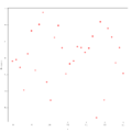
The residual analysis, in which one plots the residuals over the independent variables, provides information

• the correctness of the assumed linear relationship,
• possible outliers ,
• Homoscedasticity , heteroscedasticity .

One goal of residual analysis is to verify the premise of the residuals . It is important to note that ${\displaystyle {\hat {\varepsilon }}_{t}}$

${\displaystyle {\hat {\varepsilon }}_{t}\neq \varepsilon _{t}}$

applies. The residual can be calculated with the formula . In contrast to this, the disturbance variable cannot be calculated or observed. According to the assumptions made above, this should apply to all disturbance variables ${\displaystyle {\hat {\varepsilon }}_{t}}$ ${\displaystyle {\hat {\varepsilon }}_{t}=y_{t}-{\hat {y}}_{t}}$ ${\displaystyle \varepsilon _{t}}$

${\displaystyle \operatorname {Var} (\varepsilon _{t})=\sigma ^{2}=\mathrm {konst.} }$

There is thus a homogeneity of variance . This phenomenon is also known as homoscedasticity and can be transferred to the residuals. This means that if you plot the independent variables against the residuals , no systematic patterns should be discernible. ${\displaystyle x}$ ${\displaystyle {\hat {\varepsilon }}}$

• 

  Example 1 for residual analysis

• 

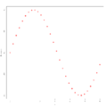
  Example 2 for residual analysis

• 

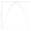
  Example 3 for residual analysis

In the three graphs above, the independent variables have been plotted against the residuals , and in example 1 it can be seen that there is actually no recognizable pattern in the residuals, i.e. This means that the assumption of homogeneity of variance is fulfilled. In Examples 2 and 3, however, this assumption is not fulfilled: a pattern can be recognized. To use linear regression, suitable transformations must therefore first be carried out here. In example 2, a pattern can be seen that is reminiscent of a sine function, with which a data transformation of the form would be conceivable here, while in example 3 a pattern can be seen that is reminiscent of a parabola, in this case one Data transformation of the form might be appropriate. ${\displaystyle x}$ ${\displaystyle {\hat {\varepsilon }}}$ ${\displaystyle a\cdot \sin(tx_{t}+c)}$ ${\displaystyle a\cdot (x_{t}-c)^{2}}$

Contribution of the individual regressors to the explanation of the dependent variables

One is interested in whether individual parameters or regressors can be removed from the regression model, i.e. whether a regressor does not (or only slightly) contribute to the explanation of . This is possible if a parameter is equal to zero, thus testing the null hypothesis . This means that you test whether the -th parameter is equal to zero. If this is the case, the associated -th regressor can be removed from the model. The vector is distributed as a linear transformation of as follows: ${\displaystyle \mathbf {y} }$ ${\displaystyle \beta _{k}}$ ${\displaystyle H_{0}\colon \beta _{k}=0}$ ${\displaystyle k}$ ${\displaystyle k}$ ${\displaystyle x_{k}}$ ${\displaystyle \mathbf {b} }$ ${\displaystyle \mathbf {y} }$

${\displaystyle \mathbf {b} \;\sim \;{\mathcal {N}}\left({\boldsymbol {\beta }},\sigma ^{2}{(\mathbf {X} ^{\top }\mathbf {X} )}^{-1}\right)}$

If one estimates the variance of the disturbance variables, one obtains for the estimated covariance matrix of the least squares estimator

${\displaystyle {\hat {\Sigma }}_{\mathbf {b} }={\hat {\sigma }}^{2}(\mathbf {X} ^{\top }\mathbf {X} )^{-1}}$.

The estimated variance of a regression parameter is the -th diagonal element in the estimated covariance matrix. The test variable results ${\displaystyle \sigma ^{2}}$ ${\displaystyle b_{k}}$ ${\displaystyle k}$

${\displaystyle t_{k}={\frac {b_{k}}{{\hat {\sigma }}_{b_{k}}}}\sim t(T-K)}$,

where the root of the estimated variance of the -th parameter represents the (estimated) standard error of the regression coefficient . ${\displaystyle {\hat {\sigma }}_{b_{k}}^{2}={\hat {\sigma }}^{2}(\mathbf {X} ^{\top }\mathbf {X} )_{kk}^{-1}}$ ${\displaystyle k}$ ${\displaystyle {\hat {\sigma }}_{b_{k}}}$

The test or pivot statistics are t-distributed with degrees of freedom. If it is greater than the critical value , the quantile of the distribution with degrees of freedom, the hypothesis is rejected. Thus the regressor is retained in the model and the contribution of the regressor in explaining is significantly large, i.e. H. significantly different from zero. ${\displaystyle T-K}$ ${\displaystyle |t_{k}|}$ ${\displaystyle t_{(1-\alpha /2,T-K)}}$ ${\displaystyle (1-\alpha /2)}$ ${\displaystyle t}$ ${\displaystyle T-K}$ ${\displaystyle x_{k}}$ ${\displaystyle x_{k}}$ ${\displaystyle y}$

forecast

A simple model for predicting endogenous variables is given by

${\displaystyle \mathbf {y} _{0}=\mathbf {X} _{0}{\boldsymbol {\beta }}+{\boldsymbol {\varepsilon }}_{0}}$,

where represents the vector of future dependent variables and the matrix of explanatory variables at the time . ${\displaystyle \mathbf {y} _{0}}$ ${\displaystyle \mathbf {X} _{0}}$ ${\displaystyle T_{0}}$

The prediction is shown as follows: from which the following prediction error results: ${\displaystyle {\hat {\mathbf {y} }}_{0}=\mathbf {X} _{0}\mathbf {b} }$ ${\displaystyle {\hat {\mathbf {y} }}_{0}-\mathbf {y} _{0}}$

Properties of the prediction error:

The average forecast error is zero: ${\displaystyle \operatorname {E} ({\hat {\mathbf {y} }}_{0}-\mathbf {y} _{0})=\operatorname {E} (\mathbf {X} _{0}(\mathbf {b} -{\boldsymbol {\beta }})-{\boldsymbol {\varepsilon }}_{0})=\mathbf {0} }$

The covariance matrix of the prediction error is: ${\displaystyle \operatorname {E} \left(({\hat {\mathbf {y} }}_{0}-\mathbf {y} _{0}-\operatorname {E} ({\hat {\mathbf {y} }}_{0}-\mathbf {y} _{0}))(({\hat {\mathbf {y} }}_{0}-\mathbf {y} _{0}-\operatorname {E} ({\hat {\mathbf {y} }}_{0}-\mathbf {y} _{0}))^{\top }\right)=\sigma ^{2}\left(\mathbf {X} _{0}(\mathbf {X} ^{\top }\mathbf {X} )^{-1}\mathbf {X} _{0}^{\top }+\mathbf {I} \right)}$

If one determines a predicted value, one might want to know in which interval the predicted values ​​move with a fixed probability. So one will determine a forecast interval for the average forecast value. In the case of linear single regression, the variance is the prediction error ${\displaystyle \operatorname {E} (\mathbf {y} _{0})}$

${\displaystyle \operatorname {Var} ({\hat {y}}_{0}-y_{0})=\sigma ^{2}\left(1+{\frac {1}{T}}+{\frac {(x_{0}-{\overline {x}})^{2}}{\sum \limits _{t=1}^{\top }(x_{t}-{\overline {x}})^{2}}}\right)}$.

The prediction interval for the variance of the prediction error is then obtained ${\displaystyle (1-\alpha )}$

${\displaystyle \left[{\hat {y}}_{0}-t_{1-\alpha /2;T-K}\cdot {\sqrt {\operatorname {Var} ({\hat {y}}_{0}-y_{0})}}\;;\;{\hat {y}}_{0}+t_{1-\alpha /2;T-K}\cdot {\sqrt {\operatorname {Var} ({\hat {y}}_{0}-y_{0})}}\right]}$.

Especially for the case of simple linear regression, the prediction interval results :

${\displaystyle \left[{\hat {y}}_{0}-t_{1-\alpha /2;T-K}\cdot {\sqrt {\sigma ^{2}\left(1+{\frac {1}{T}}+{\frac {(x_{0}-{\overline {x}})^{2}}{\sum \nolimits _{t=1}^{T}(x_{t}-{\overline {x}})^{2}}}\right)}}\;;\;{\hat {y}}_{0}+t_{1-\alpha /2;T-K}\cdot {\sqrt {\sigma ^{2}\left(1+{\frac {1}{T}}+{\frac {(x_{0}-{\overline {x}})^{2}}{\sum \nolimits _{t=1}^{T}(x_{t}-{\overline {x}})^{2}}}\right)}}\right]}$

From this form of the forecast interval one can immediately see that the forecast interval becomes wider as the exogenous forecast variable moves away from the “center of gravity” of the data. Estimates of the endogenous variables should therefore be within the observation space of the data, otherwise they will be very unreliable. ${\displaystyle x_{0}}$

The generalized model of multiple linear regression

In the generalized model of linear multiple regression , it is allowed for the structural relationship that the disturbance variables are heteroscedastic and autocorrelated. The covariance matrix of the disturbance vector is then not under the Gauss-Markow assumptions as is usually the case , but has the structure where any known real, nonsingular positive definite matrix is ​​assumed and represents a still unknown scalar. The resulting model with is called a generalized (multiple) linear regression model (with fixed regressors), or VLR for short . ${\displaystyle \mathbf {y} =\mathbf {X} {\boldsymbol {\beta }}+{\boldsymbol {\varepsilon }},}$ ${\displaystyle \operatorname {Cov} ({\boldsymbol {\varepsilon }})=\sigma ^{2}\mathbf {I} _{T}}$ ${\displaystyle \operatorname {Cov} ({\boldsymbol {\varepsilon }})=\mathbb {E} ({\boldsymbol {\varepsilon }}{\boldsymbol {\varepsilon }}^{\top })=\sigma ^{2}\mathbf {\Psi } =\mathbf {\Phi } }$ ${\displaystyle \mathbf {\Psi } }$ ${\displaystyle T\times T}$ ${\displaystyle \sigma ^{2}}$ ${\displaystyle \mathbf {y} =\mathbf {X} {\boldsymbol {\beta }}+{\boldsymbol {\varepsilon }}}$ ${\displaystyle {\boldsymbol {\varepsilon }}\sim (\mathbf {0} ,\sigma ^{2}{\boldsymbol {\Psi }})}$

Polynomial regression

Polynomial regression is a special case of multiple linear regression. The multiple linear regression model is also used to solve special (with regard to the explanatory variables) non-linear regression problems. In polynomial regression, the expected value of the dependent variable is obtained from the explanatory variable with the help of a polynomial of degree , i.e. by the function equation ${\displaystyle p>1}$

${\displaystyle \mu _{Y}=\beta _{1}+\beta _{2}x+\beta _{3}x^{2}+\ldots +\beta _{K}x^{p}}$

described. A multiple linear regression model with the regression function mentioned above is obtained if one introduces the names for the powers of . In this case one speaks of quadratic regression. ${\displaystyle x}$ ${\displaystyle x=x_{2},\,x^{2}=x_{3},\,\ldots ,\,x^{p}=x_{K}}$ ${\displaystyle p=2}$

example

To illustrate the multiple regression, the following example examines how the dependent variable : gross value added (in prices of 95; adjusted, billion euros) depends on the independent variables “gross value added by economic sector in Germany (in current prices; billion euros)”. The data can be found in the statistics portal . Since a regression model is usually calculated on the computer, this example shows how a multiple regression can be carried out with the statistical software R. ${\displaystyle y}$

variable	Description of the variables
${\displaystyle {\text{BWSb95}}}$	Gross value added at prices of 95 ( adjusted )
${\displaystyle {\text{BBLandFF}}}$	Gross value added from agriculture, forestry, fishing
${\displaystyle {\text{BBProdG}}}$	Gross value added of the manufacturing industry excluding construction
${\displaystyle {\text{BBBau}}}$	Gross value added in the construction industry
${\displaystyle {\text{BBHandGV}}}$	Gross value added from trade, hospitality and transport
${\displaystyle {\text{BBFinVerm}}}$	Gross value added through financing, rental and corporate service providers
${\displaystyle {\text{BBDienstOEP}}}$	Gross value added by public and private service providers

First you can output a scatter diagram. It shows that the total added value is obviously positively correlated with the added value of the economic areas. This can be seen from the fact that the data points in the first column of the graphic are roughly on a straight line with a positive slope. It is noticeable that the value added in the construction industry correlates negatively with the other sectors. This can be seen from the fact that the data points in the fourth column are approximately on a straight line with a negative slope.

The first step is to enter the model with all regressors in R :

lm(BWSb95~BBLandFF+BBProdG+BBBau+BBHandGV+BBFinVerm+BBDienstÖP)

Then you can output a summary of the model with all regressors in R , then you get the following list:

Residuals:
    Min     1Q      Median  3Q     Max
    −1.5465 −0.8342 −0.1684 0.5747 1.5564

Coefficients:
            Estimate Std. Error t value Pr(>|t|)
(Intercept) 145.6533 30.1373 4.833 0.000525 ***
BBLandFF      0.4952  2.4182 0.205 0.841493
BBProdG       0.9315  0.1525 6.107 7.67e−05 ***
BBBau         2.1671  0.2961 7.319 1.51e−05 ***
BBHandGV      0.9697  0.3889 2.494 0.029840 *
BBFinVerm     0.1118  0.2186 0.512 0.619045
BBDienstÖP    0.4053  0.1687 2.402 0.035086 *
---
Signif. codes: 0 '***' 0.001 '**' 0.01 '*' 0.05 '.' 0.1 ' ' 1

Residual standard error: 1.222 on 11 degrees of freedom
Multiple R-Squared: 0.9889, Adjusted R-squared: 0.9828
F-statistic: 162.9 on 6 and 11 DF, p-value: 4.306e−10

The global F test results in a test variable of . This test variable has a p value of , so the fit is significantly good. ${\displaystyle F=162{,}9}$ ${\displaystyle 4{,}306\cdot 10^{-10}}$

The analysis of the individual contributions of the variables (Coefficients table) of the regression model shows, at a significance level of , that the variables and obviously the variable cannot adequately explain. This can be seen from the fact that the associated values ​​for these two variables are relatively small, and the hypothesis that the coefficients of these variables are zero cannot be rejected. ${\displaystyle \alpha =0{,}05}$ ${\displaystyle {\text{BBLandFF}}}$ ${\displaystyle {\text{BBFinVerm}}}$ ${\displaystyle {\text{BWSb95}}}$ ${\displaystyle t}$

The variables and are barely significant. There is a particularly strong correlation (in this example ) with the variables and , which can be seen from the associated high values. ${\displaystyle {\text{BBHandGV}}}$ ${\displaystyle {\text{BBDienstOEP}}}$ ${\displaystyle y}$ ${\displaystyle {\text{BWSb95}}}$ ${\displaystyle {\text{BBProdG}}}$ ${\displaystyle {\text{BBBau}}}$ ${\displaystyle t}$

In the next step, the non-significant regressors and are removed from the model: ${\displaystyle {\text{BBLandFF}}}$ ${\displaystyle {\text{BBFinVerm}}}$

lm(BWSb95~BBProdG+BBBau+BBHandGV+BBDienstÖP)

Then you can again output a summary of the model, then you get the following list:

Residuals:
     Min      1Q       Median   3Q      Max
     −1.34447 −0.96533 −0.05579 0.82701 1.42914

Coefficients:
             Estimate Std. Error t value Pr(>|t|)
(Intercept) 158.00900 10.87649 14.528 2.05e−09 ***
BBProdG       0.93203  0.14115  6.603 1.71e−05 ***
BBBau         2.03613  0.16513 12.330 1.51e−08 ***
BBHandGV      1.13213  0.13256  8.540 1.09e−06 ***
BBDienstÖP    0.36285  0.09543  3.802 0.0022 **
---
Signif. codes: 0 '***' 0.001 '**' 0.01 '*' 0.05 '.' 0.1 ' ' 1

Residual standard error: 1.14 on 13 degrees of freedom
Multiple R-Squared: 0.9886, Adjusted R-squared: 0.985
F-statistic: 280.8 on 4 and 13 DF, p-value: 1.783e−12

This model provides a test variable of . This test variable has a p -value of , so the fit is better than in the first model. This is mainly due to the fact that all regressors are significant in the current model. ${\displaystyle F=280{,}8}$ ${\displaystyle 1{,}783\cdot 10^{-12}}$

Web links

Wikibooks: Introduction to Regression Calculation  - Learning and Teaching Materials

Commons : Linear Regression  - collection of images, videos and audio files

• Lecture notes at Ulm University

literature

• Norman R. Draper, Harry Smith: Applied Regression Analysis. Wiley, New York 1998.
• Ludwig Fahrmeir , Thomas Kneib, Stefan Lang: Regression: Models, Methods and Applications. Springer Verlag, Berlin / Heidelberg / New York 2007, ISBN 978-3-540-33932-8 .
• Dieter Urban, Jochen Mayerl: Regression analysis: theory, technology and application. 2. revised Edition. VS Verlag, Wiesbaden 2006, ISBN 3-531-33739-4 .
• G. Judge, R. Carter Hill: Introduction to the Theory and Practice of Econometrics. 1998.

Individual evidence

1. Analogous to ( argument of the maximum ), ↑ denotes the argument of the minimum ${\displaystyle \arg \min(\cdot )}$ ${\displaystyle \arg \max(\cdot )}$
2. ↑ George G. Judge, R. Carter Hill, W. Griffiths, Helmut Lütkepohl, TC Lee: Introduction to the Theory and Practice of Econometrics. 2nd Ed. John Wiley & Sons, New York / Chichester / Brisbane / Toronto / Singapore 1988, ISBN 0-471-62414-4 p. 192.
3. ^ Alvin C. Rencher, G. Bruce Schaalje: Linear models in statistics. , John Wiley & Sons, 2008, p. 143
4. ↑ Peter Hackl : Introduction to Econometrics. 2nd updated edition, Pearson, 2008., ISBN 978-3-86894-156-2 , p. 48.
5. ↑ George G. Judge, R. Carter Hill, W. Griffiths, Helmut Lütkepohl , TC Lee: Introduction to the Theory and Practice of Econometrics. 2nd Ed. John Wiley & Sons, New York / Chichester / Brisbane / Toronto / Singapore 1988, ISBN 0-471-62414-4 p. 201.
6. ↑ George G. Judge, R. Carter Hill, W. Griffiths, Helmut Lütkepohl, TC Lee: Introduction to the Theory and Practice of Econometrics. 2nd Ed. John Wiley & Sons, New York / Chichester / Brisbane / Toronto / Singapore 1988, ISBN 0-471-62414-4 p. 168.
7. ↑ George G. Judge, R. Carter Hill, W. Griffiths, Helmut Lütkepohl, TC Lee: Introduction to the Theory and Practice of Econometrics. 2nd Ed. John Wiley & Sons, New York / Chichester / Brisbane / Toronto / Singapore 1988, ISBN 0-471-62414-4 p. 266.
8. ^ Ludwig Fahrmeir , Thomas Kneib , Stefan Lang, Brian Marx: Regression: models, methods and applications. Springer Science & Business Media, 2013, ISBN 978-3-642-34332-2 , p. 109.
9. ^ Ludwig Fahrmeir, Thomas Kneib, Stefan Lang, Brian Marx: Regression: models, methods and applications. Springer Science & Business Media, 2013, ISBN 978-3-642-34332-2 , p. 109.
10. ^ Rainer Schlittgen: Regression analyzes with R. 2013, ISBN 978-3-486-73967-1 , p. 29 (accessed via De Gruyter Online).
11. ↑ Ludwig von Auer : Econometrics. An introduction. Springer, ISBN 978-3-642-40209-8 , 6th through. u. updated edition 2013, p. 135.
12. ↑ Fritz Pokropp : Linear regression and analysis of variance 2015, ISBN 978-3-486-78668-2 , page 108 (available via De Gruyter Online).
13. ↑ Werner Timischl : Applied Statistics. An introduction for biologists and medical professionals. 3. Edition. 2013, p. 342.