Angular velocity

Physical size
Surname	Angular speed, rotational speed, rotational speed
Formula symbol	${\displaystyle {\vec {\omega }}}$
Derived from	angle
Size and unit system unit dimension SI rad · s −1 T −1

The angular velocity is in the physics a vectorial quantity , which indicates how fast a angle to the time varies around an axis. Your formula symbol is (small omega ). The SI unit of angular velocity is . It plays a role in particular with rotations and is then also referred to as the rotational speed or rotational speed . In many cases in which the direction of the axis of rotation does not change in the reference system, it is sufficient to use the scalar as the amount of the vector. ${\displaystyle {\vec {\omega }}}$ ${\displaystyle {\tfrac {\mathrm {rad} }{\mathrm {s} }}}$

Definitions

Angular velocity

Angular speed and path speed of the circular motion ${\displaystyle {\vec {\omega }}}$ ${\displaystyle {\vec {v}}}$

The angular velocity is represented by a pseudo vector which indicates the direction of the axis of rotation and the speed of the rotational movement. The direction of the pseudo-vector is oriented in such a way that it indicates the direction of rotation according to the corkscrew rule. The magnitude of the angular velocity is equal to the derivative of the angle of rotation with respect to time : ${\displaystyle {\vec {\omega }}}$ ${\displaystyle \omega =\left|{\vec {\omega }}\right|}$ ${\displaystyle \varphi }$ ${\displaystyle t}$

${\displaystyle \omega ={\frac {\mathrm {d} \varphi }{\mathrm {d} t}}}$

Therefore, at constant angular velocity, the following applies

${\displaystyle \omega ={\frac {2\pi }{T}}}$,

because in the period of rotation the angle 2 is traversed. ${\displaystyle T}$ ${\displaystyle \pi }$

In the case of a plane circular movement, the direction of the current path speed of a point changes with the same angular speed as the radius vector of the point. In the case of a path curve curved in space, this applies to the current circle of curvature. The change in the direction of the path velocity can therefore just as easily be used to define the angular velocity. It results directly from the data of the path and does not require the determination of an axis of rotation.

The magnitude of the angular velocity is mostly used for operations in which the axis of rotation does not change. A change in the direction and / or amount of the angular velocity is the result of an angular acceleration . ${\displaystyle \omega }$

Track speed

Each point of the rotating system describes a circular path, the plane of which is perpendicular to the axis of rotation. The orbit or speed of rotation of the point on this circle is according to the amount ${\displaystyle {\vec {v}}}$

${\displaystyle v=\omega \,r_{\perp }}$,

where is the radius of the circular motion. Because the infinitesimal way belongs to the infinitesimal time span . ${\displaystyle r_{\perp }}$ ${\displaystyle \mathrm {d} t}$ ${\displaystyle \mathrm {d} s=r_{\perp }\,\mathrm {d} \varphi =r_{\perp }\,\omega \,\mathrm {d} t}$

If the origin of the coordinate system lies on the axis of rotation, then the path speed in terms of direction and amount is equal to the cross product of the angular speed and the position vector: ${\displaystyle O}$

${\displaystyle {\vec {v}}={\vec {\omega }}\times {\vec {r}}}$,

because the distance from the axis is

${\displaystyle r_{\perp }=r\,\mathrm {sin} \vartheta }$

with the polar angle , which indicates the constant angular distance between the axis of rotation and the position vector to the point under consideration. ${\displaystyle \vartheta }$

This consideration of the rate of change of the position vector applies to every vector that is subject to rotation, e.g. B. for the basis vectors ( ) of a rotating reference system . Their rate of change is ${\displaystyle {\vec {e}}'_{i}}$ ${\displaystyle i\in \{x,y,z\}}$

${\displaystyle {\frac {\mathrm {d} {\vec {e}}'_{i}}{\mathrm {d} t}}\,=\,{\vec {\omega }}\times {\vec {e}}'_{i}}$.

Delimitation to the angular frequency

→ Main article : angular frequency

Although the angular frequency and the angular velocity are denoted by the same symbol and even though they are measured in the same unit, they are two different physical quantities. ${\displaystyle \omega }$

The angular velocity indicates the rate of change of a geometric angle and is used in connection with rotary movements.

The angular frequency, on the other hand, is an abstract quantity in the context of vibrations. An oscillation can be represented mathematically by a rotating pointer (see pointer model ). The angle of the pointer is called the phase or phase angle. The rate of change of this phase angle is the angular frequency. So it is - like the frequency  - a measure of how fast an oscillation takes place and - apart from the rotation of the imaginary pointer - has nothing to do with a rotary movement.

Angular velocity of the line of sight

Level movement

The angular velocity of the line of sight from the origin O to the particle P is determined by the tangential velocity of the velocity vector v.

The velocity vector v of a particle P relative to an observer O can be broken down into polar coordinates . The radial component of the velocity vector does not change the direction of the line of sight . The relationship between the tangential component and the angular velocity of the line of sight is:

${\displaystyle \mathrm {v} _{\perp }={\frac {d\phi }{dt}}\,r=\omega \cdot r}$

It should be noted that the angular velocity of the line of sight depends on the (arbitrarily) chosen location of the observer.

Spatial movement

In three dimensions, the angular velocity is characterized by its magnitude and its direction.

As in the two-dimensional case, the particle has one component of its velocity vector in the direction of the radius vector and another perpendicular to it. The plane with the support vector (location of the observer) and direction vectors and defines a plane of rotation in which the behavior of the particle appears for a moment as in the two-dimensional case. The axis of rotation is then perpendicular to this plane and defines the direction of the vector of the instantaneous angular velocity. Radius and velocity vectors are assumed to be known. The following then applies: ${\displaystyle {\vec {0}}}$ ${\displaystyle {\vec {r}}}$ ${\displaystyle {\vec {v}}_{\perp }}$

${\displaystyle {\vec {\omega }}={\frac {{\vec {r}}\times {\vec {v}}}{|{\vec {r}}|^{2}}}}$

Here, too, the angular velocity calculated in this way depends on the (arbitrarily) selected location of the observer. For example, in cylindrical coordinates (ρ, φ, z) with and calculated from this, we get : ${\displaystyle {\vec {r}}={\begin{pmatrix}\rho \cos \varphi \\\rho \sin \varphi \\z\end{pmatrix}}}$ ${\displaystyle {\vec {v}}={\frac {d}{dt}}{\vec {r}}}$

${\displaystyle ({\rho }^{2}+z^{2}){\vec {\omega }}={\dot {\rho }}z{\hat {e}}_{\varphi }+{\dot {\varphi }}(-z\rho {\hat {e}}_{\rho }+\rho ^{2}{\hat {e}}_{z})-{\dot {z}}\rho {\hat {e}}_{\varphi }}$

Here, the basis vectors to cylindrical coordinates . ${\displaystyle {\hat {e}}_{\rho },{\hat {e}}_{\varphi },{\hat {e}}_{z}}$

In spherical coordinates (r, θ, φ) it follows analogously . ${\displaystyle {\vec {\omega }}=-{\dot {\varphi }}\sin \theta {\hat {e}}_{\theta }+{\dot {\theta }}{\hat {e}}_{\varphi }}$

One application is the relative movement of objects in astronomy (see proper movement (astronomy) ).

Angular velocity with special approaches to movement

When rotating bodies, angles can be used to parameterize the movement. A selection of frequently used approaches is described below.

Euler angles in the z-y'-x '' convention

Rotation of the position angle from the earth's fixed coordinate system ( English world frame , Index g) to the fixed body coordinate system ( English body frame , Index f)

In vehicle or aircraft construction, the orientation of the vehicle-mounted system is specified in Euler angles relative to the earth-mounted system . Three consecutive rotations are standardized. First around the z-axis of the system g (yaw angle), then around the y-axis of the rotated system (pitch angle) and finally around the x-axis of the body-fixed coordinate system (roll / roll angle).

The angular velocity of the system fixed to the body results from the angular velocities around these axes.

${\displaystyle {\vec {\omega }}={\dot {\psi }}{\vec {\mathbf {u} }}_{1}+{\dot {\theta }}{\vec {\mathbf {u} }}_{2}+{\dot {\phi }}{\vec {\mathbf {u} }}_{3}}$

The added point denotes the time derivative. This basis is not orthonormal. The unit vectors can, however , be calculated with the aid of elementary rotations.

Euler angles in the z-x'-z '' convention

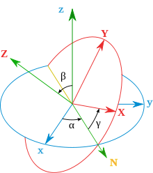
Euler's base system (green) indicates the axes around which the Euler angles α, β and γ rotate.

In the standard x-convention (z, x ', z' ') , see figure, rotation is first carried out with the angle α around the fixed z-axis, then with the angle β around the x-axis in its position according to the first rotation (x'-axis, in the picture the N-axis) and finally with the angle γ around the z-axis in its position after the two previous rotations (symbol z '', in the picture the Z-axis).

If the unit vectors designate the space-fixed standard basis (blue in the picture), then the angular velocity with respect to the space-fixed basis reads ${\displaystyle {\hat {e}}_{x,y,z}}$

${\displaystyle {\begin{aligned}{\vec {\omega }}=&{\dot {\alpha }}{\hat {e}}_{z}+{\dot {\beta }}[\cos(\alpha ){\hat {e}}_{x}+\sin(\alpha ){\hat {e}}_{y}]+{\dot {\gamma }}[\sin(\alpha )\sin(\beta ){\hat {e}}_{x}-\cos(\alpha )\sin(\beta ){\hat {e}}_{y}+\cos(\beta ){\hat {e}}_{z}]\\=&[{\dot {\beta }}\cos(\alpha )+{\dot {\gamma }}\sin(\alpha )\sin(\beta )]{\hat {e}}_{x}+[{\dot {\beta }}\sin(\alpha )-{\dot {\gamma }}\cos(\alpha )\sin(\beta )]{\hat {e}}_{y}+[{\dot {\alpha }}+{\dot {\gamma }}\cos(\beta )]{\hat {e}}_{z}.\end{aligned}}}$

In the moving base (red in the picture) this results in the same meaning: ${\displaystyle {\hat {e}}_{X,Y,Z}}$

${\displaystyle {\begin{aligned}{\vec {\omega }}=&{\dot {\alpha }}[\sin(\beta )\sin(\gamma ){\hat {e}}_{X}+\sin(\beta )\cos(\gamma ){\hat {e}}_{Y}+\cos(\beta ){\hat {e}}_{Z}]+{\dot {\beta }}[\cos(\gamma ){\hat {e}}_{X}-\sin(\gamma ){\hat {e}}_{Y}]+{\dot {\gamma }}{\hat {e}}_{Z}\\=&[{\dot {\alpha }}\sin(\beta )\sin(\gamma )+{\dot {\beta }}\cos(\gamma )]{\hat {e}}_{X}+[{\dot {\alpha }}\sin(\beta )\cos(\gamma )-{\dot {\beta }}\sin(\gamma )]{\hat {e}}_{Y}+[{\dot {\alpha }}\cos(\beta )+{\dot {\gamma }}]{\hat {e}}_{Z},\end{aligned}}}$

see motion function of the symmetrical top .

Cylindrical coordinates

In the cylindrical coordinate system (ρ, φ, z) the basis vectors are

${\displaystyle {\hat {e}}_{\rho }={\begin{pmatrix}\cos \varphi \\\sin \varphi \\0\end{pmatrix}},\quad {\hat {e}}_{\varphi }={\begin{pmatrix}-\sin \varphi \\\cos \varphi \\0\end{pmatrix}},\quad {\hat {e}}_{z}={\begin{pmatrix}0\\0\\1\end{pmatrix}}.}$

If the angle φ changes, the angular velocity arises . It is used to calculate the rates of the basis vectors, for example ${\displaystyle {\vec {\omega }}={\dot {\varphi }}{\hat {e}}_{z}}$ ${\displaystyle {\dot {\hat {e}}}_{\rho }={\vec {\omega }}\times {\hat {e}}_{\rho }.}$

This results from the Euler angles in the z-x'-z '' convention with

• α = φ and β = γ ≡ 0 or
• γ = φ and α = β ≡ 0.

Spherical coordinates

In spherical coordinates (r, φ, θ) the basis vectors

${\displaystyle {\hat {e}}_{r}={\begin{pmatrix}\sin \theta \cos \varphi \\\sin \theta \sin \varphi \\\cos \theta \end{pmatrix}},\qquad {\hat {e}}_{\theta }={\begin{pmatrix}\cos \theta \cos \varphi \\\cos \theta \sin \varphi \\-\sin \theta \end{pmatrix}},\qquad {\hat {e}}_{\varphi }={\begin{pmatrix}-\sin \varphi \\\cos \varphi \\0\end{pmatrix}}}$

to be used. With a common rotation of these basis vectors with variable angles φ and θ , the angular velocity arises

${\displaystyle {\vec {\omega }}={\begin{pmatrix}-{\dot {\theta }}\sin \varphi \\{\dot {\theta }}\cos \varphi \\{\dot {\varphi }}\end{pmatrix}}={\dot {\varphi }}\cos \theta {\hat {e}}_{r}-{\dot {\varphi }}\sin \theta {\hat {e}}_{\theta }+{\dot {\theta }}{\hat {e}}_{\varphi }.}$

With it the rates of the basis vectors are calculated, for example according to ${\displaystyle {\dot {\hat {e}}}_{\theta }={\vec {\omega }}\times {\hat {e}}_{\theta }.}$

This results from the Euler angles in the z-x'-z '' convention with α ≡ 0, β = φ and γ = θ as well as the cyclic exchange of the coordinate directions 123 _Euler → 312 _sphere .

Angular velocity tensors

Rotation of a vector around the axis of rotation with an angle by an orthogonal tensor . ${\displaystyle {\vec {v}}}$ ${\displaystyle {\vec {n}}}$ ${\displaystyle \alpha }$ ${\displaystyle \mathbf {Q} }$

Definition of the angular velocity tensor

The cross product of the angular velocity with the position vector can be viewed as the vector transformation of the position vector by the angular velocity tensor.

Because a pure rotation of vectors is represented by orthogonal tensors , that is, orthogonal mappings of vectors on vectors:, see picture. Here, Q is the orthogonal tensor with the property ( 1 is the unit tensor , the superscript T denotes the transposition ) and is the vector onto which the fixed vector is mapped. Time derivative gives: ${\displaystyle {\vec {x}}=\mathbf {Q} \cdot {\vec {X}}}$ ${\displaystyle \mathbf {Q\cdot Q} ^{\top }=\mathbf {Q^{\top }\cdot Q} =\mathbf {1} }$ ${\displaystyle {\vec {x}}}$ ${\displaystyle {\vec {X}}}$

${\displaystyle {\dot {\vec {x}}}={\dot {\mathbf {Q} }}\cdot {\vec {X}}={\dot {\mathbf {Q} }}\cdot \mathbf {Q} ^{\top }\cdot {\vec {x}}=:\mathbf {\Omega } \cdot {\vec {x}}}$

The angular velocity tensor Ω occurring here is skew-symmetrical ( Ω ^┬ = - Ω ) because of

${\displaystyle {\dot {\mathbf {1} }}={\frac {\mathrm {d} }{\mathrm {d} t}}(\mathbf {Q\cdot Q} ^{\top })={\dot {\mathbf {Q} }}\cdot \mathbf {Q} ^{\top }+\mathbf {Q} \cdot {\dot {\mathbf {Q} }}^{\top }=\mathbf {\Omega +\Omega } ^{\top }=\mathbf {0} \,.}$

Angular velocity tensor and angular velocity

Every skew symmetric tensor W has a dual vector with the property for all . In the case of the angular velocity tensor, this dual vector is the angular velocity: ${\displaystyle {\vec {w}}}$ ${\displaystyle \mathbf {W} \cdot {\vec {x}}={\vec {w}}\times {\vec {x}}}$ ${\displaystyle {\vec {x}}}$

${\displaystyle {\dot {\vec {x}}}=\mathbf {\Omega } \cdot {\vec {x}}={\vec {\omega }}\times {\vec {x}}\,.}$

The dual vector

${\displaystyle {\vec {\omega }}=-{\frac {1}{2}}\sum _{i=1}^{3}\sum _{j=1}^{3}\Omega _{ij}{\hat {e}}_{i}\times {\hat {e}}_{j}}$

is the negative half of the vector invariant of the tensor and as such is an axial vector . The coordinates Ω _{ij of} the tensor Ω belong to the standard basis ${\displaystyle {\hat {e}}_{1,2,3}.}$

Conversely, the angular velocity tensor can be obtained from the angular velocity:

${\displaystyle {\begin{aligned}\mathbf {\Omega } =&{\vec {\omega }}\times \mathbf {1} :=\sum _{i=1}^{3}\omega _{i}{\hat {e}}_{i}\times \sum _{k=1}^{3}{\hat {e}}_{k}\otimes {\hat {e}}_{k}:=\sum _{i=1}^{3}\sum _{k=1}^{3}\omega _{i}({\hat {e}}_{i}\times {\hat {e}}_{k})\otimes {\hat {e}}_{k}={\begin{pmatrix}0&-\omega _{3}&\omega _{2}\\\omega _{3}&0&-\omega _{1}\\-\omega _{2}&\omega _{1}&0\end{pmatrix}}\\\rightarrow \mathbf {\Omega } \cdot {\vec {x}}=&({\vec {\omega }}\times \mathbf {1} )\cdot {\vec {x}}:={\vec {\omega }}\times (\mathbf {1} \cdot {\vec {x}})={\vec {\omega }}\times {\vec {x}},\end{aligned}}}$

see. Cross product matrix . The arithmetic symbol " " forms the dyadic product . ${\displaystyle \otimes }$

Angular velocity tensor for rotating vector space bases

The angular velocity tensor can be calculated directly from the rates of vectors of a vector space basis that performs a rigid body rotation. ${\displaystyle {\vec {g}}_{1,2,3}}$

Because the tensor , in which the basis vectors are entered in columns, is invertible according to the assumption: ${\displaystyle \mathbf {G} :=\sum _{i=1}^{3}{\vec {g}}_{i}\otimes {\hat {e}}_{i}}$

${\displaystyle |\mathbf {G} |={\begin{vmatrix}{\vec {g}}_{1}&{\vec {g}}_{2}&{\vec {g}}_{3}\end{vmatrix}}\cdot {\begin{vmatrix}{\hat {e}}_{1}&{\hat {e}}_{2}&{\hat {e}}_{3}\end{vmatrix}}\neq 0.}$

The vertical lines represent the determinant , the non-disappearance of which guarantees invertibility. In the case of a common rigid body rotation of the basis vectors it follows:

${\displaystyle {\dot {\vec {g}}}_{1,2,3}={\vec {\omega }}\times {\vec {g}}_{1,2,3}\quad \leftrightarrow \quad {\dot {\mathbf {G} }}={\vec {\omega }}\times \mathbf {G} =\mathbf {\Omega \cdot G} \quad \leftrightarrow \quad \mathbf {\Omega } ={\dot {\mathbf {G} }}\cdot \mathbf {G} ^{-1}}$

Conversely, if the time derivative of a tensor G, multiplied by its inverse G ⁻¹ , is skew symmetrical, then the column vectors of the tensor can be interpreted as a rotating basis. In the event that the vectors form an orthonormal basis , the tensor G is orthogonal and the relationship already mentioned results ${\displaystyle {\vec {g}}_{1,2,3}}$ ${\displaystyle \mathbf {\Omega } ={\dot {\mathbf {G} }}\cdot \mathbf {G} ^{\top }.}$

Exponential of the angular velocity tensor

If the angular velocity is constant, the angular velocity tensor is also constant. Then, given the initial value G (t = 0), it can be integrated over time with the result: ${\displaystyle {\dot {\mathbf {G} }}=\mathbf {\Omega \cdot G} }$

${\displaystyle \mathbf {G} (t)=\exp(\mathbf {\Omega } t)\cdot \mathbf {G} (t=0).}$

For the first four powers of Ω are calculated using the BAC-CAB formula to

${\displaystyle {\begin{aligned}{\vec {\omega }}=&\omega {\hat {n}}\quad {\text{mit}}\quad |{\hat {n}}|=1\\\mathbf {\Omega } =&\omega {\hat {n}}\times \mathbf {1} =\omega n_{i}{\hat {e}}_{i}\times {\hat {e}}_{j}\otimes {\hat {e}}_{j}\\\mathbf {\Omega } ^{2}=&(\omega n_{i}{\hat {e}}_{i}\times {\hat {e}}_{j}\otimes {\hat {e}}_{j})\cdot (\omega n_{k}{\hat {e}}_{k}\times {\hat {e}}_{l}\otimes {\hat {e}}_{l})=\omega ^{2}n_{i}n_{k}{\hat {e}}_{i}\times ({\hat {e}}_{k}\times {\hat {e}}_{l})\otimes {\hat {e}}_{l}\\=&\omega ^{2}n_{i}n_{k}(\delta _{il}{\hat {e}}_{k}-\delta _{ik}{\hat {e}}_{l})\otimes {\hat {e}}_{l}=\omega ^{2}n_{k}{\hat {e}}_{k}\otimes n_{i}{\hat {e}}_{i}-\omega ^{2}n_{i}n_{i}{\hat {e}}_{l}\otimes {\hat {e}}_{l}=-\omega ^{2}(\mathbf {1} -{\hat {n}}\otimes {\hat {n}})\\\mathbf {\Omega } ^{3}=&-\omega {\hat {n}}\times \mathbf {1} \cdot \omega ^{2}(\mathbf {1} -{\hat {n}}\otimes {\hat {n}})=-\omega ^{3}[{\hat {n}}\times \mathbf {1} \cdot \mathbf {1} -({\hat {n}}\times \mathbf {1} \cdot {\hat {n}})\otimes {\hat {n}}]=-\omega ^{3}{\hat {n}}\times \mathbf {1} \\\mathbf {\Omega } ^{4}=&\omega ^{2}({\hat {n}}\otimes {\hat {n}}-\mathbf {1} )\cdot \omega ^{2}({\hat {n}}\otimes {\hat {n}}-\mathbf {1} )=\omega ^{4}({\hat {n}}\otimes {\hat {n}}-{\hat {n}}\otimes {\hat {n}}-{\hat {n}}\otimes {\hat {n}}+\mathbf {1} )=\omega ^{4}(\mathbf {1} -{\hat {n}}\otimes {\hat {n}})\end{aligned}}}$

Above, Einstein's summation convention is to be used, according to which indices from one to three that occur twice in a product are to be summed up. After complete induction , the potencies result

${\displaystyle {\begin{aligned}\mathbf {\Omega } ^{2k}=&(-1)^{k}\omega ^{2k}(\mathbf {1} -{\hat {n}}\otimes {\hat {n}})\\\mathbf {\Omega } ^{2k+1}=&(-1)^{k}\omega ^{2k+1}{\hat {n}}\times \mathbf {1} \end{aligned}}}$

for k = 1, 2, 3, ... (no sums) With the definition Ω ⁰  : = 1 , the exponential exp of the angular velocity tensor can be determined with the Taylor series :

${\displaystyle {\begin{aligned}\exp(\mathbf {\Omega } t):=&\sum _{k=0}^{\infty }{\frac {(\mathbf {\Omega } t)^{k}}{k!}}=\mathbf {1} +\sum _{k=1}^{\infty }{\frac {(\mathbf {\Omega } t)^{2k}}{(2k)!}}+\sum _{k=0}^{\infty }{\frac {(\mathbf {\Omega } t)^{2k+1}}{(2k+1)!}}\\=&\mathbf {1} +\sum _{k=1}^{\infty }{\frac {(-1)^{k}(\omega t)^{2k}}{(2k)!}}(\mathbf {1} -{\hat {n}}\otimes {\hat {n}})+\sum _{k=0}^{\infty }{\frac {(-1)^{k}(\omega t)^{2k+1}}{(2k+1)!}}{\hat {n}}\times \mathbf {1} \\=&\mathbf {1} +[\cos(\omega t)-1](\mathbf {1} -{\hat {n}}\otimes {\hat {n}})+\sin(\omega t){\hat {n}}\times \mathbf {1} \end{aligned}}}$

The last equation represents an orthogonal tensor. If Ω is only defined as a skew symmetric tensor without the cross product, this can be generalized to rotations in n dimensions .

Angular velocity of the rigid body

The angular velocity of a rotating rigid body is clear, because the direction of the orbital velocity reverses once at all points in the same period of rotation . The angular velocity is also independent of the choice of the location of the axis of rotation to which the rotation is related. Angular velocities are commutative with respect to addition; that is, they can be summed like vectors. (This does not apply to finite rotations.) Every point of a rigid body has the same angular velocity vector. ${\displaystyle 2\pi }$

Uniqueness

Proof of the independence of the angular velocity from the choice of the reference point

The rigid body may rotate around any axis. It is shown that the angular velocity is independent of the choice of the reference point through which the axis passes. This means that the angular velocity is an independent property of the rotating rigid body.

The origin of the laboratory system is in O, while O ₁ and O _{2 are} two points on the rigid body with velocities and respectively . Assuming that the angular velocity is relative to O ₁ or O ₂ , or since points P and O ₂ each have only one velocity, the following applies: ${\displaystyle {\vec {v}}_{1}}$ ${\displaystyle {\vec {v}}_{2}}$ ${\displaystyle {\vec {\omega }}_{1}}$ ${\displaystyle {\vec {\omega }}_{2}.}$

${\displaystyle {\vec {v}}_{1}+{\vec {\omega }}_{1}\times {\vec {r}}_{1}={\vec {v}}_{2}+{\vec {\omega }}_{2}\times {\vec {r}}_{2}}$

${\displaystyle {\vec {v}}_{2}={\vec {v}}_{1}+{\vec {\omega }}_{1}\times {\vec {r}}={\vec {v}}_{1}+{\vec {\omega }}_{1}\times ({\vec {r}}_{1}-{\vec {r}}_{2})}$

Substituting the lower equation for into the upper one gives: ${\displaystyle {\vec {v}}_{2}}$

${\displaystyle ({\vec {\omega }}_{1}-{\vec {\omega }}_{2})\times {\vec {r}}_{2}={\vec {0}}}$

Since the point P (and thus ) can be chosen arbitrarily, it follows: ${\displaystyle {\vec {r}}_{2}}$

${\displaystyle {\vec {\omega }}_{1}={\vec {\omega }}_{2}}$

The angular velocity of the rigid body is therefore independent of the choice of the reference point of the axis of rotation. Thus, for example, the measurement of the yaw rate in a vehicle is independent of the installation location of the yaw rate sensor .

Commutativity

As the time interval becomes smaller, the quadrangle (black) converges to a flat parallelogram , and the difference between the two speeds tends to zero. ${\displaystyle {\dot {\vec {x}}}_{12},\ {\dot {\vec {x}}}_{21}}$

Although rotations may generally not be interchanged in their order, the commutativity of the addition is given in the case of the angular velocity. It does not matter in which order the components of the angular velocity or entire angular velocity vectors are added (unlike rotations, see picture).

Mathematically this can be shown by rotations with two angular velocities in an (infinitesimal) small time interval d t . In the time interval d t a particle moving at the site after . Another rotation with the angular velocity supplies the end position and the shift ${\displaystyle {\vec {x}}}$ ${\displaystyle {\vec {x}}'={\vec {x}}+{\vec {\omega }}_{1}\times {\vec {x}}\,\mathrm {d} t}$ ${\displaystyle {\vec {\omega }}_{2}}$ ${\displaystyle {\vec {x}}''={\vec {x}}'+{\vec {\omega }}_{2}\times {\vec {x}}'\,\mathrm {d} t}$

${\displaystyle {\begin{aligned}\mathrm {d} {\vec {x}}_{12}:=&{\vec {x}}''-{\vec {x}}={\vec {x}}'+{\vec {\omega }}_{2}\times {\vec {x}}'\,\mathrm {d} t-{\vec {x}}\\=&({\vec {x}}+{\vec {\omega }}_{1}\times {\vec {x}}\,\mathrm {d} t)+{\vec {\omega }}_{2}\times ({\vec {x}}+{\vec {\omega }}_{1}\times {\vec {x}}\,\mathrm {d} t)\,\mathrm {d} t-{\vec {x}}\\=&{\vec {\omega }}_{1}\times {\vec {x}}\,\mathrm {d} t+{\vec {\omega }}_{2}\times {\vec {x}}\,\mathrm {d} t+{\vec {\omega }}_{2}\times ({\vec {\omega }}_{1}\times {\vec {x}})\,\mathrm {d} t^{2}.\end{aligned}}}$

The limit value d t → 0 can be calculated:

${\displaystyle {\dot {\vec {x}}}_{12}=\lim _{\mathrm {d} t\to 0}{\frac {\mathrm {d} {\vec {x}}_{12}}{\mathrm {d} t}}=({\vec {\omega }}_{1}+{\vec {\omega }}_{2})\times {\vec {x}}}$

This speed corresponds to a rotation with the angular speed . If the order of the infinitesimal rotations is reversed, an identical result is derived for the speed . This is why angular velocities add up like vectors and infinitesimally small rotations - unlike large rotations - can be interchanged in their order. ${\displaystyle {\vec {\omega }}_{1}+{\vec {\omega }}_{2}}$ ${\displaystyle {\dot {\vec {x}}}_{21}}$

Proof with tensor calculus

Rotations can be described with orthogonal tensors, two of which, Q 1,2 , are given. With the definitions ${\displaystyle {\begin{aligned}\mathbf {\Omega } _{k}:=&{\dot {\mathbf {Q} }}_{k}\cdot \mathbf {Q} _{k}^{\top }\\{\bar {\mathbf {\Omega } }}_{k}:=&\mathbf {Q} _{k}^{\top }\cdot {\dot {\mathbf {Q} }}_{k}=\mathbf {Q} _{k}^{\top }\cdot \mathbf {\Omega } _{k}\cdot \mathbf {Q} _{k}\end{aligned}}}$ for k = 1, 2 the speed of a vector , which results from the rotation of the fixed vector , is calculated as: ${\displaystyle {\vec {x}}_{21}=\mathbf {Q} _{1}\cdot \mathbf {Q} _{2}\cdot {\vec {X}}}$ ${\displaystyle {\vec {X}}}$ ${\displaystyle {\begin{aligned}{\dot {\vec {x}}}_{21}=&({\dot {\mathbf {Q} }}_{1}\cdot \mathbf {Q} _{2}+\mathbf {Q} _{1}\cdot {\dot {\mathbf {Q} }}_{2})\cdot {\vec {X}}\\=&\mathbf {Q} _{1}\cdot (\mathbf {Q} _{1}^{\top }\cdot {\dot {\mathbf {Q} }}_{1}+{\dot {\mathbf {Q} }}_{2}\cdot \mathbf {Q} _{2}^{\top })\cdot \mathbf {Q} _{2}\cdot {\vec {X}}\\=&\mathbf {Q} _{1}\cdot ({\bar {\mathbf {\Omega } }}_{1}+\mathbf {\Omega } _{2})\cdot \mathbf {Q} _{2}\cdot {\vec {X}}\end{aligned}}}$ If the order of the rotations is reversed, the generally different speed results analogously ${\displaystyle {\vec {x}}_{12}=\mathbf {Q} _{2}\cdot \mathbf {Q} _{1}\cdot {\vec {X}},}$ ${\displaystyle {\dot {\vec {x}}}_{12}=({\dot {\mathbf {Q} }}_{2}\cdot \mathbf {Q} _{1}+\mathbf {Q} _{2}\cdot {\dot {\mathbf {Q} }}_{1})\cdot {\vec {X}}=\mathbf {Q} _{2}\cdot ({\bar {\mathbf {\Omega } }}_{2}+\mathbf {\Omega } _{1})\cdot \mathbf {Q} _{1}\cdot {\vec {X}}\,.}$ These identities apply to rotations of any size. Calculation of the velocities in the state Q 1,2 = 1 provides the angular velocities at the location Then and the above equations specialize ${\displaystyle {\vec {x}}:={\vec {x}}_{12}={\vec {x}}_{21}={\vec {X}}.}$ ${\displaystyle {\bar {\mathbf {\Omega } }}_{1,2}=\mathbf {\Omega } _{1,2}}$ ${\displaystyle {\begin{aligned}{\dot {\vec {x}}}_{21}=&(\mathbf {\Omega } _{1}+\mathbf {\Omega } _{2})\cdot {\vec {x}}=({\vec {\omega }}_{1}+{\vec {\omega }}_{2})\times {\vec {x}}\\{\dot {\vec {x}}}_{12}=&(\mathbf {\Omega } _{2}+\mathbf {\Omega } _{1})\cdot {\vec {x}}=({\vec {\omega }}_{2}+{\vec {\omega }}_{1})\times {\vec {x}}\,,\end{aligned}}}$ see angular velocity tensor and angular velocity . Because the addition of tensors is commutative, the velocities agree: ${\displaystyle {\dot {\vec {x}}}_{21}={\dot {\vec {x}}}_{12}={\vec {v}}=({\vec {\omega }}_{1}+{\vec {\omega }}_{2})\times {\vec {x}}=({\vec {\omega }}_{2}+{\vec {\omega }}_{1})\times {\vec {x}}}$

Thus the commutativity of the addition of the angular velocities is proven.

Applications and examples

The angular velocity occurs in many equations and applications in physics, astronomy or technology .

• A celestial body moving at a distance R from the earth with speed perpendicular to the line of sight shows an apparent angular speed in the sky . With meteors (shooting stars) it can be up to 90 ° per second, very close small planets or comets can move a few degrees per hour in the sky. For stars, the angular velocity is given in angular seconds per year and called proper motion . ${\displaystyle v_{t}}$ ${\displaystyle \mu =v_{t}/R}$

• According to Kepler's third law , the squares of the periods of revolution T of the planets behave like the third powers of the major semiaxes a of their orbits. The angular velocities behave like (“Kepler rotation”). According to Kepler's second law, the angular velocity of a planet in an elliptical orbit in relation to the sun depends on the respective distance and thus varies along the orbit. It is greatest when the planet is in perihelion and smallest when it is in aphelion . ${\displaystyle \omega \propto 1/a^{3/2}}$

• When a rigid body rotates around a fixed axis, the angular velocity ω, in contrast to the velocity v, is independent of the radius. Its rotational energy and its angular momentum are functions of its angular velocity.

• The angular speed of a rotor in an electric motor , which rotates constantly at 3,000 revolutions per minute, is

${\displaystyle \omega =2\pi \cdot 3000\cdot {\tfrac {1}{60\,{\text{s}}}}=314{,}16\,{\tfrac {\text{rad}}{\text{s}}}.}$

When specifying speeds , units such as and are also used, see the article speed . ${\displaystyle \mathrm {\tfrac {U}{min}} }$ ${\displaystyle \mathrm {\tfrac {1}{min}} }$

• Let be the angular frequency of the harmonic oscillation of a pendulum with the amplitude . Then the angular velocity of the pendulum is calculated as a function of time: ${\displaystyle \omega _{0}}$ ${\displaystyle {\hat {\varphi }}}$

${\displaystyle \omega (t)={\dot {\varphi }}(t)={\frac {d}{dt}}[{\hat {\varphi }}\cdot \sin(\omega _{0}t)]={\hat {\varphi }}\cdot \omega _{0}\cdot \cos(\omega _{0}t)}$

• In the case of airplanes or cars , the angular velocities are specified in components of the vehicle-fixed coordinate system. According to the x, y and z components, we speak of roll / roll speed, pitch speed, yaw speed. More information can be found
  • in flight under roll axis , transverse axis , yaw axis and
  • in vehicle construction under driving dynamics .

literature

The angular velocity is dealt with in many textbooks and formulas in the natural and engineering sciences.

• Horst Stöcker: Pocket book of physics . 6th edition. Harri Deutsch, 2010, ISBN 978-3-8171-1860-1 .
• Lothar Papula: Mathematics for Engineers and Natural Scientists 1 . 12th edition. Vieweg + Teubner, 2009, ISBN 978-3-8348-0545-4 .

Individual evidence

1. ↑ Manfred Knaebel, Helmut Jäger, Roland Mastel: Technical Schwingungslehre . Springer-Verlag, 2009, ISBN 978-3-8351-0180-7 , p. 8th ff . ( books.google.com. ).
2. ↑ Jürgen Eichler: Physics. Basics for engineering studies - short and to the point . Springer DE, 2011, ISBN 978-3-8348-9942-2 , pp. 112 , urn : nbn: de: 1111-20110310734 ( limited preview in Google Book search).
3. ^ Institute for Physics at the University of Rostock (Ed.): Theoretical Physics II - Theoretical Mechanics . Chapter 5 - Rigid Body and Top Theory. S. 109 ( Page no longer available , search in web archives: online [accessed June 6, 2017]).