Lagrange top

Fig. 1: Realization of a Lagrange gyro

The Lagrange top is a heavy symmetrical top with a support point, which and the center of mass lie on its figure axis , so that the weight exerts a torque on it. A typical gyroscopic motion is shown in Fig. 1.

Joseph-Louis Lagrange was the first to solve the associated equations of motion in 1788, which is why Lagrange's name is associated with this top. Compared to the force-free Euler top , the Lagrange top is particularly relevant due to the omnipresent gravity on earth. In terms of gyroscopic theory, it is closely related to the frictionless game top .

The line of a point on the body axis, in short the Locuskurve, resembles a cycloid and can have tips or loops, see Fig. 3 to 5 . Special forms of movement of the Lagrange top are regular precession , in which the top circles uniformly around the vertical, see Figs. 1, 7 and 8 . The pseudoregular precession cannot be distinguished from the regular precession with the naked eye, but it carries out rapid oscillations on a small-scale level. The regular or pseudoregular precession with a horizontal figure axis, which the top can maintain against its weight , appears paradoxical , see Fig. 2 . The movement of the vertically hanging top is always stable; in the vertically upright position, a critical angular velocity must be exceeded for stability . In this case, the top does not leave the vertical without cause and is called a sleeping top . The Lagrange top that does not rotate around its figure axis is a spherical pendulum that is only touched at the edge here.

The movements of the Lagrange top are one of the three always integrable cases , along with those of the Euler and Kowalewskaja tops . In particular, the locus curve can be examined analytically and thus provides information about the gyroscopic movement and its stability against disturbances.

The Lagrange top is realized by a typical toy top when its touchdown point is freely rotatable on the ground as in the animation, a limitation that is discussed when comparing the play top with the Lagrange top .

Designations on the Lagrange top

Every Lagrange top has three degrees of freedom for which the precession angle ψ , the inclination angle ϑ and the intrinsic rotation φ are used in gyro theory , see Euler angle in gyro theory . The Lagrange top is a symmetrical top with a figure axis , where the terms equatorial plane , equatorial moment of inertia and axial moment of inertia can be looked up. The perpendicular direction of gravity is the vertical or perpendicular precession axis and the parallel upward axis denotes the z-direction. The precession axis and the figure axis span the precession plane . The node line or node axis is perpendicular to the precession plane, see also node (astronomy) . Likewise, the moment of weight is perpendicular to the precession plane, because the Lagrange top has the center of gravity on the figure axis, which lies in the precession plane. The node axis is oriented in such a way that it is parallel to the moment of weight in the same direction.

With an upright or raised top, the figure axis points upwards, thus forming an obtuse angle with the weight , while with a hanging or lowered top this angle is acute and the top hangs down.

Classification of Lagrange tops

Lagrange tops differ in terms of top theory only in three sizes:

1. the axial moment of inertia C  = Θ ₃ around the figure axis,
2. the equatorial moment of inertia A  = Θ ₁  = Θ ₂ about perpendicular axes and
3. the support point moment c ₀  =  mg s , which results from the distance s between support point and center of gravity and the weight mg of the top.

During the movement of the Lagrange top, the following quantities remain constant, which are called integrals in top theory :

Total energy E of the top

It is made up of the positional and rotational energy . The earth's gravitational field is conservative and the gyroscopic motion thus obeys the law of conservation of energy .

Angular momentum L _z around the plumb line

This is constant because the plumb line is parallel to the weight, the moment of which therefore cannot change the angular momentum L _z .

Axial angular momentum L ₃ around the figure axis

This is constant because the center of gravity of the Lagrange top is by definition on the figure axis and the moment of weight is perpendicular to its lever arm , which here points from the base to the center of gravity. Therefore the end point of the angular momentum vector can only move in one plane perpendicular to the figure axis, see also angular velocity and angular momentum for a symmetrical top . The component L ₃ is therefore constant in the body-fixed system.

Dissipative influences such as friction are neglected, if not explicitly mentioned. All Lagrangian tops that match in A, C, c ₀ , E, L _z and L ₃ and start from the same starting position show identical behavior.

Homologous tops

To analyze the locus curve, it is sufficient to consider spherical gyroscopes with A  = Θ ₁  = Θ ₂  = Θ ₃  =  C , whose moments of inertia are therefore equal to the equatorial moment of inertia A of a gyro of interest. Because all gyroscopes that have the same angular momentum and match in terms of A, c ₀ and a constant k , which combines potential and kinetic energies, show the same locus curves with the same starting position. These similar gyroscopes - and this also includes said spherical gyroscopes - are called homologous to each other . The analysis of spherical tops is simpler and more general in this regard. However, the common features of all homologous Lagrange tops are limited to the locus curve and in particular do not include the intrinsic rotation angle φ about the figure axis . However, the difference in the corresponding intrinsic speed of rotation between two homologous gyroscopes is always constant. Gaston Darboux first noticed these similarities in the gyroscopic movements .

Phenomenology of gyrations

Representation of the locus curve

Central to the discussion of the movements of a Lagrange top is the locus curve on which the point of intersection of the figure axis through the unit sphere moves around the support point, the locus of the figure axis. Designations from geography are adopted on this sphere as a guide: The upper dead point is in the north pole and the lower dead point in the south pole of the sphere. The horizontal plane through the support point intersects the sphere at the equator and a small circle of the sphere parallel to it is called the circle of latitude . Half a great circle that connects the North Pole and South Pole is called the meridian .

To illustrate the Locuskurven of hanging gyros in Figures 3 and 4 one was stereographic projection used. The projection center is above the support point × and the image plane in the north pole of the sphere.

Alternatively, perspective views as in Fig. 5 are also used.

The gyroscopic effect of the axial angular momentum

Fig. 2: Spoked wheel precessing horizontally in a circle (along the red ellipse R) (bold black)

When moving the Lagrange top, the axial angular momentum L ₃ follows the figure axis . According to the principle of twist , when the direction of the figure axis changes, a gyroscopic effect arises that is exactly the opposite of this movement.

This mechanism enables the paradoxical movement of the horizontal top, in which the figure axis moves in the horizontal plane, see Fig. 2. Here the said top effect is oriented horizontally and when it is just so large that it balances the always horizontal moment of the weight force , the figure axis remains in the horizontal. The condition for this particular regular precession is L _z  ·  L ₃  =  A · c ₀ , see # Regular precession .

In general, however, the gyroscopic action has a horizontal and a vertical component. The latter is not compensated for by any external moment, so that the top is deflected by the vertical top effect. The top deviates until a dynamic equilibrium with the weight is found in the horizontal one .

Locus curves as a function of L ₃

• 

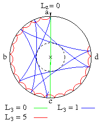
  Fig. 3: Locus curves without vertical angular momentum

• 

  Fig. 4: Locus curves with negative vertical angular momentum

Fig. 3 shows gyroscopic movements without vertical angular momentum, where the orbit around the south pole is exclusively caused by the gyroscopic effect described above. In the case L ₃  = 0, the top corresponds to a spherical pendulum that swings back and forth between points a, the south pole and c (vertical green line). With increasing axial angular momentum, the figure's axis is deflected more and more in the direction of movement to the right. If L _{3 is} greater than about 10, the arcs that are passed through become so small that they can no longer be recognized as such with the eye. This movement, which then appears regularly, is called pseudoregular precession and leads here along the equator abcd.

The spherical pendulum receives an angular momentum L _z  = -0.3, see Fig. 4, green curve, through a rotary shock in a horizontal direction in a clockwise direction . At L ₃  = - L _z the top swings through the south pole (yellow curve). The loops that occur at L ₃  > - L _z also become  so small here with L ₃ > 10 that they are no longer recognizable as such with the eye and the top shows a pseudoregular precession along the equator. If the gyroscope receives an angular momentum L ₃  <- L _z , then it is deflected so far to the left in the direction of movement that it misses the bottom dead center. At he can walk in regular precession along the equator adcb (black circle). Below this value is the locus curve in the northern hemisphere, where it initially shows waves, later peaks and finally loops. From L ₃  <-10 these loops are again so small that a pseudoregular precession takes place along the equator. ${\displaystyle L_{3}={\tfrac {Ac_{0}}{L_{z}}}=-3{\tfrac {1}{3}}}$

Locus curves as a function of L _z

Fig. 5: Locus curves of an upright Lagrange top

Figure 5 shows locus curves of an upright Lagrange top, the movement of which begins with the black arrow. The locus curves show loops (purple and yellow), peaks (light red and light blue) or waves (green). At L _z ≈ 2.53 a slow regular precession takes place (blue circle of latitude). With increasing L _z > L _3, the loops wrap around the north pole and the sphere further and further and approach the blue circle of latitude from the north, in which a rapid regular precession then finally takes place. A further increase in L _z yields ever larger loops that touch the blue parallel from the south and a more southerly parallel from the north. With L _z → ∞ the southern tangent circle of latitude approaches the blue circle of latitude mirrored at the equator and the locus curve becomes a great circle that is tangent to these two circles of latitude.

If the angular momentum is sufficiently large and aligned close to the figure axis, a pseudoregular precession also takes place with the upright top.

Pseudoregular precession

→ Main article : Pseudoregular precession

The pseudoregular precession is the most important point of the theory of the Lagrange gyro and has attracted the greatest interest in natural philosophy because of the frequency of its occurrence and its paradoxical properties . Phenomenology shows that the locus curve of the Lagrange gyro often moves between two circles of latitude. With pseudoregular precession, the two parallels approach each other so far without collapsing that they can no longer be separated from one another with the eye. The movement then looks like a regular precession, but it is not and is called a pseudoregular precession . The regular precession can only arise with very specific initial conditions, whereas the pseudoregular allows any initial conditions as long as the initial angular momentum L is aligned close to the figure axis and is sufficiently large, i.e. about L ²> 100  A c ₀ .

Because the figure axis is only near the angular momentum vector, it quickly revolves around it on a narrow cone. These tremors on the figure axis are called nutations after a word borrowed from astronomy . The rotation of the figure axis of a top around the angular momentum vector can be approximated to the unit sphere by a cycloid in a tangential plane, which can be looked up in the main article.

Fast Lagrangian top

With a fast top, its rotational energy dominates over its potential energy. If the angular velocity around the figure axis is increased n-fold with the same initial conditions of the gyro, then the trajectory of the gyro is identical to that of the gyro with the original angular velocity, but at which the gravitational acceleration was divided by n². In the former case of high angular velocity, the trajectory is traversed n times faster. Correspondingly, the fast heavy top shows asymptotically the same behavior for ω → ∞ as the force-free Euler top .

Analytical description of the movement

Movement function of the Lagrange top

For the analytical solution of the equations of motion, the gyroscopic motion is represented with Euler angles ψ, ϑ and φ , see Euler angles in gyroscopic theory . With their time derivatives , the angular velocity , the total energy and the constant angular momentum around the figure axis and the plumb line can be expressed. So there are three equations at three unknown angles, which in this case allow the angle of inclination wobei to be calculated, resulting in elliptical integrals that are solved by elliptical functions.

For the angle ϑ , the constant and u  : = cos ϑ results in the autonomous differential equation ${\displaystyle k:=2AE+\left(1-{\tfrac {A}{C}}\right)L_{3}^{2}}$

${\displaystyle {\dot {u}}^{2}=U(u):={\frac {1}{A^{2}}}[(k-L_{3}^{2}-2c_{0}Au)(1-u^{2})-(L_{z}-L_{3}u)^{2}]}$

The gyro function U is a third degree polynomial in u . In the physically relevant area, U (u) ≥ 0 and | u | Be ≤ 1. If L ₃ and L _z are equal in terms of amount, u  = 1 or u  = -1 is a zero of U and thus the figure axis can reach the vertical. If L _z  ≠  L ₃ , because U (1) <0 and U (∞)> 0 a zero is greater than one. The sign of results from the usual procedure for vibrations. The variable u moves in the interval [-1, 1] between two extremes, between which the polynomial U is positive and in which U  = 0. Its sign changes in these zeros . ${\displaystyle {\dot {u}}}$ ${\displaystyle {\dot {u}}}$

The motion function follows after separating the variables:

${\displaystyle {\begin{aligned}t(\vartheta )=&\int {\frac {\mathrm {d} u}{\sqrt {U(u)}}}\\\psi (\vartheta )=&\int {\underline {\frac {L_{z}-L_{3}u}{A(1-u^{2})}}}{\frac {\mathrm {d} u}{\sqrt {U(u)}}}\\\varphi (\vartheta )=&\int {\underline {\left[{\frac {L_{3}-L_{z}u}{A(1-u^{2})}}+L_{3}\left({\frac {1}{C}}-{\frac {1}{A}}\right)\right]}}{\frac {\mathrm {d} u}{\sqrt {U(u)}}}\end{aligned}}}$

The fraction is equal to the differential of time d t and the underlined terms are the angular velocities at angles ψ and φ . The angle ϑ results from the inverse of the function t (ϑ) . On the right-hand side there are so-called elliptic integrals whose solutions are elliptic functions . ${\displaystyle {\tfrac {\mathrm {d} u}{\sqrt {U(u)}}}}$

The choice of the sign of the root in the denominators of the integrands depends on the integration interval. When integrating over an interval [ u ₀ , u ₁ ] without zeros, the sign of the difference u ₁ - u ₀ must be taken for the root in the denominators . That is why the integrals over an interval [ u ₀ , u ₁ ] give the same result as when integrating over the interval [ u ₁ , u ₀ ]. This explains the symmetry properties of the locus curves, which are composed of pieces that are congruent or mirror images of one another.

The angle of inclination ϑ is calculated specifically

${\displaystyle {\begin{aligned}\cos \vartheta =&u=u_{0}+(u_{1}-u_{0})\operatorname {sn} ^{2}\left({\sqrt {\frac {c_{0}(u_{2}-u_{0})}{2A}}}(t-t_{0});k\right)\\K(k)=&\int _{0}^{\frac {\pi }{2}}{\frac {\mathrm {d} x}{\sqrt {1-k^{2}\sin ^{2}(x)}}}\\T=&2K(k){\sqrt {\frac {2A}{c_{0}(u_{2}-u_{0})}}}\end{aligned}}}$

Here sn ( z; k ) are the Jacobian elliptic function sinus amplitudinis , u _{0,1,2 are} the three zeros of the gyro function sorted according to size and the elliptic module . The dimensionless elliptic module occurs only in the complete elliptic integral K and the elliptic function sn and must not be confused with the kinetic constant k , which has the dimension M ² L ⁴ T  ^–2 . The function of n ( z k ), the period 4 K and the angle θ , the period T . This time elapses between two contacts between the Locus curve and the southern parallel at . The angles ψ and φ result as a linear combination of two Legendre integrals Π of the third kind . ${\displaystyle k:={\sqrt {\tfrac {u_{1}-u_{0}}{u_{2}-u_{0}}}}}$ ${\displaystyle \cos \vartheta =u_{0}}$

Derivation of the autonomous differential equation

With the Euler angles in gyro theory , the vector components and angular velocities are expressed and inserted into the constants: ${\displaystyle {\begin{aligned}L_{3}=&C\omega _{3}=C({\dot {\psi }}\cos(\vartheta )+{\dot {\varphi }})\\L_{z}=&(A\omega _{1}{\hat {e}}_{1}+A\omega _{2}{\hat {e}}_{2}+C\omega _{3}{\hat {e}}_{3})_{z}=A{\dot {\psi }}\sin ^{2}(\vartheta )+L_{3}\cos(\vartheta )\end{aligned}}}$ The indices 1, 2 and 3 refer to the main axis system. So the angles ψ and φ result as a function of the angle ϑ : ${\displaystyle {\begin{aligned}{\dot {\psi }}=&{\frac {L_{z}-L_{3}\cos(\vartheta )}{A\sin ^{2}(\vartheta )}}\\{\dot {\varphi }}=&{\frac {L_{3}}{C}}-{\dot {\psi }}\cos(\vartheta )=L_{3}\left({\frac {1}{C}}-{\frac {1}{A}}\right)+{\frac {L_{3}-L_{z}\cos(\vartheta )}{A\sin ^{2}(\vartheta )}}\end{aligned}}}$ The total energy can now be represented as a function of the angle ϑ alone : ${\displaystyle {\begin{aligned}2E=&A\omega _{1}^{2}+A\omega _{2}^{2}+C\omega _{3}^{2}+2c_{0}\cos(\vartheta )\\=&A{\dot {\psi }}^{2}\sin(\vartheta )^{2}+A{\dot {\vartheta }}^{2}+{\frac {L_{3}^{2}}{C}}+2c_{0}\cos(\vartheta )\\\rightarrow {\dot {\vartheta }}^{2}=&{\frac {2E}{A}}-{\frac {L_{3}^{2}}{AC}}-{\frac {2c_{0}}{A}}\cos(\vartheta )-{\frac {[L_{z}-L_{3}\cos(\vartheta )]^{2}}{A^{2}\sin ^{2}(\vartheta )}}\end{aligned}}}$ With the substitution ${\displaystyle u:=\cos(\vartheta )\rightarrow {\dot {u}}=-{\dot {\vartheta }}\sin(\vartheta )\rightarrow {\dot {\vartheta }}^{2}={\frac {{\dot {u}}^{2}}{\sin ^{2}(\vartheta )}}={\frac {{\dot {u}}^{2}}{1-u^{2}}}}$ and the constant becomes it ${\displaystyle k:=2AE+\left(1-{\tfrac {A}{C}}\right)L_{3}^{2}}$ ${\displaystyle {\dot {u}}^{2}=U(u):={\frac {1}{A^{2}}}[(k-L_{3}^{2}-2c_{0}Au)(1-u^{2})-(L_{z}-L_{3}u)^{2}]}$ After separating the variables with the above expressions for , the movement can be represented with the mentioned elliptic integrals for t, ψ and φ as a function of the angle ϑ , the solutions of which are elliptic functions . ${\displaystyle {\dot {\psi }},{\dot {\varphi }}}$

Representation of the angle of inclination with elliptical functions
Representation of the angle of inclination with the sinus amplitudinis sn
The gyro function is expressed by its three zeros u 0,1,2 , for which -1 <  u 0  <  u 1  <+1 <  u 2 is assumed: ${\displaystyle {\dot {u}}^{2}=U(u)={\frac {2c_{0}}{A}}(u-u_{0})(u-u_{1})(u-u_{2})}$ In the range -∞ <u ≤  u 0 and u 1  ≤ u <  u 2 , the gyro function is negative, otherwise positive. In the interval u  ∈ [  u 0 , u 1 ] the substitution yields the factors ${\displaystyle \sin ^{2}(v):={\tfrac {u-u_{0}}{u_{1}-u_{0}}}}$ ${\displaystyle {\begin{aligned}u-u_{0}=&(u_{1}-u_{0})\sin ^{2}(v)\\u-u_{1}=&-(u_{1}-u_{0})\cos(v)^{2}\\u-u_{2}=&-(u_{2}-u_{0})\left(1-{\frac {u_{1}-u_{0}}{u_{2}-u_{0}}}\sin ^{2}(v)\right)\end{aligned}}}$ and with the elliptical module (not to be confused with the kinetic constant k ) the time derivatives ${\displaystyle k^{2}={\tfrac {u_{1}-u_{0}}{u_{2}-u_{0}}}}$ ${\displaystyle {\begin{aligned}{\dot {u}}=&{\sqrt {U(u)}}=(u_{1}-u_{0})\sin(v)\cos(v){\sqrt {{\frac {2c_{0}}{A}}(u_{2}-u_{0})\left(1-k^{2}\sin ^{2}(v)\right)}}\\{\frac {\mathrm {d} }{\mathrm {d} t}}\sin ^{2}(v)=&2\sin(v)\cos(v){\dot {v}}={\frac {\dot {u}}{u_{1}-u_{0}}}\\\rightarrow {\dot {v}}=&{\sqrt {{\frac {c_{0}}{2A}}(u_{2}-u_{0})\left(1-k^{2}\sin ^{2}(v)\right)}}\end{aligned}}}$ After separating the variables, this leads to the Legendre form of an elliptic integral of the first kind : ${\displaystyle {\begin{aligned}z(v):=&\int _{0}^{v}{\frac {\mathrm {d} \vartheta }{\sqrt {1-k^{2}\sin(\vartheta )^{2}}}}={\sqrt {{\frac {c_{0}}{2A}}(u_{2}-u_{0})}}(t-t_{0})\end{aligned}}}$ It was assumed here that the gyro starts at time t 0 at the latitude u = u 0 , i.e. with . The Jacobian elliptic function sn has the property sn ( z (v); k ) = sin ( v ) which gives the solution function in the text. ${\displaystyle v=0}$
Representation of the angle of inclination with the Weierstrasse ℘ function
The differential equation can be expressed using the form ${\displaystyle {\dot {u}}^{2}=U(u)}$ ${\displaystyle u={\sqrt[{3}]{\tfrac {2A}{c_{0}}}}x+{\tfrac {k}{6Ac_{0}}}}$ ${\displaystyle {\dot {x}}^{2}=4x^{3}-g_{2}x-g_{3}}$ bring, which is fulfilled by the Weierstrasse function . Are in it ${\displaystyle {\begin{aligned}g_{2}=&-{\frac {k^{2}+12A^{2}c_{0}^{2}-12AL_{3}L_{z}c_{0}}{\sqrt[{3}]{108A^{8}c_{0}^{4}}}}\\g_{3}=&-{\frac {k^{3}-18Ac_{0}k(2Ac_{0}+L_{3}L_{z})+54A^{2}c_{0}^{2}(L_{z}^{2}+L_{3}^{2})}{54A^{4}c_{0}^{2}}}\end{aligned}}}$ Constants of motion.

Creation of waves, peaks and loops in the locus curve

As already explained in the section #Motion function of the Lagrange gyro , a zero point of the gyro function is greater than one. Only the other two zeros u _1,2  = cos ϑ _1,2 can determine the locus, which is located between two extremes. In these extremes the gyro function vanishes ( U  = 0.)

Due , the zero e of the numerator, with L _z - L ₃ e = 0, determines the shape of the locus curve: ${\displaystyle {\dot {\psi }}={\tfrac {L_{z}-L_{3}u}{A(1-u^{2})}}}$

1. If e lies outside the physically achievable range, then everywhere is or and the locus curve is wavy and resembles a shortened cycloid. ${\displaystyle {\dot {\psi }}<0}$ ${\displaystyle {\dot {\psi }}>0}$
2. If e is within the physically achievable area, then the sign changes there and the locus curve resembles an elongated cycloid with loops. ${\displaystyle {\dot {\psi }}}$
3. If e coincides with one of the zeros of U , then is there and the locus curve appears like an ordinary cycloid with peaks. This corresponds to the case where the figure axis is released from rest. ${\displaystyle {\dot {\psi }}={\dot {\vartheta }}=0}$

Regular precession

→ Main article : Regular precession

In regular precession, ϑ is just like u and the angular velocities are constant. With the angular momentum components ${\displaystyle {\dot {\psi }},{\dot {\varphi }}}$

${\displaystyle {\vec {L}}=L_{v}{\hat {e}}_{z}+L_{f}{\hat {e}}_{3},\;L_{v}={\frac {L_{z}-L_{3}u}{1-u^{2}}},\;L_{f}={\frac {L_{3}-L_{z}u}{1-u^{2}}}}$

it occurs when

${\displaystyle Ac_{0}=L_{v}L_{f}={\frac {L_{z}-L_{3}u}{1-u^{2}}}{\frac {L_{3}-L_{z}u}{1-u^{2}}}}$

That is written in the Euler angles

${\displaystyle C{\dot {\psi }}{\dot {\varphi }}+(C-A){\dot {\psi }}^{2}u=c_{0}}$

In regular precession, the constants meet this condition. The condition is symmetrical in L ₃ and L _z , because the condition remains fulfilled when the two angular impulses exchange their values. The equations of motion cannot be solved in regular precession with the elliptic integrals above, because the integration intervals have zero expansion. However, the angular velocities can be directly integrated because they are constant ${\displaystyle {\dot {\psi }},{\dot {\vartheta }},{\dot {\varphi }}}$

${\displaystyle {\begin{aligned}\vartheta =&\arccos(u)\\\psi =&{\frac {L_{z}-L_{3}u}{A(1-u^{2})}}t+\psi _{0}\\\varphi =&L_{3}\left({\frac {1}{C}}-{\frac {1}{A}}\right)t+{\frac {L_{3}-L_{z}u}{A(1-u^{2})}}t+\varphi _{0}\end{aligned}}}$

wherein ψ ₀ and φ ₀ adapting to initial conditions at t  serve = 0th

Regular precession is a stable form of movement.

Slow and fast regular precession or nutation

• 

  Fig. 7: Fast regular precession

• 

  Fig. 8: Slow regular precession

For a given direction cosine u and angular momentum L ₃ around the figure axis, there are at most two angular velocities that are compatible with regular precession. ${\displaystyle {\dot {\psi }}}$

Because then the condition is because of a quadratic equation in with the solutions: ${\displaystyle c_{0}=C{\dot {\psi }}{\dot {\varphi }}+(C-A){\dot {\psi }}^{2}u}$ ${\displaystyle {\dot {\varphi }}=\omega _{3}-{\dot {\psi }}u}$ ${\displaystyle {\dot {\psi }}}$

${\displaystyle {\dot {\psi }}_{1,2}={\frac {L_{3}}{2Au}}\left(1\pm {\sqrt {1-{\frac {4c_{0}Au}{L_{3}^{2}}}}}\right)\approx {\begin{cases}{\frac {L_{3}}{Au}}\\{\frac {c_{0}}{L_{3}}}\end{cases}}}$

The right approximation applies to the fast gyro , where is. The fast precession in the first case corresponds to the nutation of the force-free Euler gyroscope , which is proportional to the axial angular momentum, see Fig. 7. In the slow precession in the second case, the precession speed is inversely proportional to the axial angular momentum, see Fig. 8. ${\displaystyle L_{3}^{2}\gg 4Ac_{0}u}$

Euler-Poisson equations

→ Main article : Euler-Poisson equations

The Euler-Poisson equations are the specific equations of motion for heavy gyroscopes . Under use of Euler angles , the Poisson equations are identically satisfied and the Euler equations to specialize in Lagrange gyroscope

${\displaystyle {\begin{aligned}c_{0}\sin(\vartheta )\cos(\varphi )=&A{\dot {\omega }}_{1}+(C-A)\omega _{2}\omega _{3}\\-c_{0}\sin(\vartheta )\sin(\varphi )=&A{\dot {\omega }}_{2}+(A-C)\omega _{3}\omega _{1}\\0=&C{\dot {\omega }}_{3}\end{aligned}}}$

In this, c ₀  =  m g s is the support point moment resulting from the weight m g and the distance s of the center of gravity from the support point on the figure axis. Onset of angular velocities

${\displaystyle {\begin{aligned}\omega _{1}=&{\dot {\psi }}\sin(\vartheta )\sin(\varphi )+{\dot {\vartheta }}\cos(\varphi )\\\omega _{2}=&{\dot {\psi }}\sin(\vartheta )\cos(\varphi )-{\dot {\vartheta }}\sin(\varphi )\\\omega _{3}=&{\dot {\psi }}\cos(\vartheta )+{\dot {\varphi }}\end{aligned}}}$

and their time derivatives yield differential equations of the second order in the angles:

${\displaystyle {\begin{aligned}{\ddot {\psi }}=&{\frac {-2A{\dot {\psi }}\cos(\vartheta )+C({\dot {\varphi }}+{\dot {\psi }}\cos(\vartheta ))}{A\sin(\vartheta )}}{\dot {\vartheta }}={\frac {-2A{\dot {\psi }}\cos(\vartheta )+C\omega _{3}}{A\sin(\vartheta )}}{\dot {\vartheta }}\\{\ddot {\vartheta }}=&{\frac {(A-C){\dot {\psi }}^{2}\cos(\vartheta )-C{\dot {\psi }}{\dot {\varphi }}+c_{0}}{A}}\sin(\vartheta )={\frac {A{\dot {\psi }}^{2}\cos(\vartheta )-C\omega _{3}{\dot {\psi }}+c_{0}}{A}}\sin(\vartheta )\\{\ddot {\varphi }}=&{\dot {\psi }}{\dot {\vartheta }}\sin(\vartheta )-{\ddot {\psi }}\cos(\vartheta )\end{aligned}}}$

The angular accelerations are proportional to the angular velocity . Where the angle ϑ is momentarily stationary - as for example in regular precession - the angular velocities are constant. ${\displaystyle {\ddot {\psi }},{\ddot {\varphi }}}$ ${\displaystyle {\dot {\vartheta }}}$ ${\displaystyle {\dot {\psi }},{\dot {\varphi }}}$

Vertical Lagrangian top

In the case of a vertical Lagrangian top, the figure axis is initially parallel to the plumb line and the locus for the upright top is at the highest point, or for the hanging top at the lowest point of the unit sphere. At these points, L _z  = ± L _3, depending on whether the figure axis is parallel or antiparallel to the perpendicular direction. Accordingly, these gyroscopes have the square of the angular momentum

${\displaystyle |{\vec {L}}|^{2}=L^{2}=L_{z}^{2}=L_{3}^{2}=C^{2}\omega _{3}^{2}}$

Vertical upright gyro

Fig. 9: Locus curve (red) with its vertical projection onto the horizontal plane (blue) for the upright top

For a top that rotates at top dead center, L _z  =  L ₃ . The upright top only rotates around the figure axis at top dead center and the top function is simplified

${\displaystyle {\dot {u}}^{2}=U(u)={\frac {2c_{0}}{A}}\left(u+{\frac {2Ac_{0}-L^{2}}{2Ac_{0}}}\right)(1-u)^{2}}$

The top  can rotate continuously around the top dead center u = 1. If

L ²  > 4  A c ₀

is, then under real circumstances U  ≤ 0 and the top can  not leave the vertical u = 1 without external influences. Such a top is called a sleeping top and its movement is stable.

After a while, the angular momentum can decrease so much as a result of friction that L ²  <4  A c ₀ . Then the top dead center becomes an unstable equilibrium position and the top can break out of the vertical. In the event of a slight impact, the top leaves top dead center, drops to the latitude with it and returns. For this movement to the latitude e and back to the starting point near the top dead center, the locus curve can be calculated analytically: ${\displaystyle u={\tfrac {L^{2}-2Ac_{0}}{2Ac_{0}}}=:e}$

${\displaystyle \psi =\arctan {\sqrt {\frac {u-e}{1+e}}}+{\frac {1}{2}}{\sqrt {\frac {1+e}{1-e}}}\ln {\frac {{\sqrt {1-e}}+{\sqrt {u-e}}}{{\sqrt {1-e}}-{\sqrt {u-e}}}}}$

Here arctan is the arc tangent and ln is the natural logarithm . The curve is a kind of spherical logarithmic spiral that is tangent to the circle of latitude e and winds infinitely often around the top dead center, see Fig. 9.

Vertically hanging top

With a gyro that rotates around bottom dead center, L _z  = - L ₃ and the gyro function is simplified to

${\displaystyle {\dot {u}}^{2}=U(u)=-{\frac {1}{A^{2}}}[2Ac_{0}(1-u)+L^{2}](1+u)^{2}}$

 The gyro can rotate continuously around the bottom dead center u = -1. However, because U does not become positive under any real circumstances, the rotating Lagrange top hanging vertically downwards cannot leave the plumb line without external influences. The bottom dead center is in any case a stable equilibrium position.

This is in contrast to the uniformly rotating conical pendulum , in which the bottom dead center becomes unstable at a critical speed. There, however, the angular velocity around the plumb line is kept artificially constant, which is not the case with the Lagrange top left to its own devices. As soon as it deviates minimally from the plumb line, the pendulum is continuously supplied with angular momentum until a position is found in which the moment of centrifugal force is in equilibrium with the moment of weight force.

Stability analysis

In contrast to the Euler gyro , the stability of the movement of the Lagrange top has to be checked individually for each of its movements. The trajectories of the gyro are compared with and without disturbance. If the trajectories are adjacent, the form of motion is considered stable, otherwise it is unstable.

The stability often results from clear considerations, as for example with the regular precession. In regular precession, the gyro function has a double zero and the two circles of latitude, between which the tip of the gyro normally moves, lie on top of one another. If the gyro is disturbed, the circles of latitude move apart a little, but in any case, the less the smaller the disturbance turns out to be. Correspondingly, the top moves into a movement that differs less from the original the less the disturbance was. This proves that the regular precession of the Lagrange top is a stable movement. This applies at least as long as the double zero is not at the limits of the physically accessible interval [-1,1]. The vertical top needs special treatment. The disruption of the gyro can be assumed to be one or more of the variables L ₃ , L _z or E.

If there is an unstable position, which is, however, almost stable, as for example with a vertically hanging top, if L ²  - 4 A c _{0 is} only slightly negative, then the movement can still be stable. It is then theoretically unstable but practically stable . The reason for this is that a small perturbation ε is assumed in the stability analysis and it is then often assumed that terms of higher order in ε can be neglected. However, if the unstable position is also a stable position in an ε environment, then the smallness of the disturbance is no longer sufficient to keep the error in the assumptions made small.

Influence of friction

With the fast gyro, the influence of friction can be estimated approximately. The influence depends on the type of mounting of the top , of which the cardanic suspension and the embedding of the top of the top in a cone that is open at the top are common.

Cardanic suspension

The friction in the pivot bearings of the suspension cause the following:

• With pseudoregular precession, the nutations become smaller and eventually disappear, so that the movement turns into a regular precession.
• The axial angular momentum is constantly decreasing.
• The precession speed increases because it is inversely proportional to the axial angular momentum.
• The angle of inclination ϑ increases so that the figure axis lowers.
• The gyroscopic motion comes to a standstill at some point.

If the angular momentum decreases so much that the top ceases to be faster before the figure axis points noticeably downwards, the effect of the friction becomes more complex.

Spinning top dancing in a cone pan

This case is based on the assumption that the figure axis ends in a hemisphere in the support point, which is located in the tip of a conical funnel that is open at the top and is held there by the force of weight. The base is here in the center of the hemisphere, which slides in the cone when the top rotates. The frictional force acts approximately perpendicular to the precession plane in the horizontal direction and opposite to the tangential speed of the points of contact on the hemisphere. Correspondingly, the frictional force exerts a torque which is oriented approximately horizontally in the plane of precession and which forms an obtuse angle with the axis of the figure . This frictional torque has an axial and an equatorial component with respect to the gyro. The axial component incessantly reduces the axial angular momentum, which then increases the precession speed again. The equatorial component in the precession plane raises or lowers the figure axis, depending on whether the center of gravity of the top is higher or lower than the support point. If it is higher, as usual, then the top of the top approaches the plumb line in an Archimedean spiral in time . In contrast to the cardanic suspension, the gyro stands up here. ${\displaystyle t={\tfrac {L_{3}}{c_{0}}}\sin \vartheta }$

Web links

• K. Lüders, RO Pohl, G. Beuermann, K. Samwer: Precession of a rotating wheel. ( MP4 ) Institute for Scientific Film (IWF) , 2003, accessed on December 5, 2019 (film about a wheel precessing with a horizontal axis of rotation.). 

Footnotes

1. ↑ Grammel (1920), p. 88, Grammel (1950), p. 78, Magnus (1971), p. 109, Arnold (1988), p. 188, Leimanis (1965), p. 25.
2. ↑ Joseph-Louis Lagrange : Analytical Mechanics . Tome Second. Corucier, Paris 1815, p. 265 f . (French, archive.org [accessed August 20, 2017] Original title: Mécanique Analytique .). or Joseph-Louis Lagrange: Analytical Mechanics . Vandenhoeck and Ruprecht, Göttingen 1797 ( archive.org [accessed on August 20, 2017] German translation by Friedrich Murhard).
   
   
3. ↑ Klein and Sommerfeld (2010), p. 201.
4. ↑ ^{a b} Arnol'd (1988), p. 155.
5. ↑ Grammel (1920), p. 48.
6. ↑ Grammel (1920), p. 89.
7. ↑ Magnus (1971), p. 110, Grammel (1920), p. 95.
8. ↑ Gaston Darboux : About the movement of a heavy rotationally symmetrical body that is fixed by a point on its axis. In: Journal de mathématiques pures et appliquées . tome 1, série 4. Elsevier, 1885, ISSN  0021-7824 , p. 403 - 430 (French, mathdoc.fr [accessed on January 8, 2020] Original title: Sur le mouvement d'un corps pesant de révolution, fixé par un point de son ax . The relationship between the symmetrical and spherically symmetrical tops is found in the first Part, pp. 404 - 406.).
9. ↑ Klein and Sommerfeld (2010), p. 204 f.
10. ↑ ^{a b} Simulated locus curves with A = c ₀  = 1, cos ϑ ₀  = 0.
11. ↑ Simulated locus curves with A = c ₀  = 1, cos ϑ ₀  = 0.8.
12. ↑ Klein and Sommerfeld (2010), p. 255 f.
13. ↑ Klein u. Sommerfeld (2010), p. 209.
14. ↑ ^{a b} Magnus (1971), p. 120.
15. ↑ Klein and Sommerfeld (2010), p. 291 f.
16. ↑ Grammel (1920), p. 63 ff.
17. ↑ ^{a b} Arnol'd (1988), p. 161 ff.
18. ↑ K. Magnus (1971), p. 122, R. Grammel (1920), p. 104.
19. ↑ ^{a b} Klein and Sommerfeld (2010), p. 222 f.
20. ↑ Magnus (1971), p. 113.
21. ↑ Klein and Sommerfeld (2010), p. 267 f.
22. ↑ Magnus (1971), p. 111.
23. ↑ Grammel (1950), p. 263 ff.
24. ↑ Michèle Audin: Remembering Sofya Kovalevskaya . Springer Verlag, London a. a. 2008, ISBN 978-0-85729-928-4 , pp. 89 ff ., doi : 10.1007 / 978-0-85729-929-1 ( limited preview in the Google book search).
25. ↑ Christian Sommer: Mechanics of the rigid body. Graz University of Technology, January 27, 2003, accessed on February 23, 2018 . 
26. ↑ Magnus (1971), p. 51.
27. ↑ Grammel (1920), p. 109, Magnus (1971), p. 123.
28. ↑ Grammel (1920), p. 107, Magnus (1971), p. 124.
29. ↑ Grammel (1920), p. 110.
30. ↑ Grammel (1920), p. 111.
31. ↑ Grammel (1920), p. 106, Klein and Sommerfeld (2010), p. 289 f.
32. ^ For example, Klein and Sommerfeld (2010), p. 317 or Grammel (1920), p. 108.
33. ↑ Klein and Sommerfeld (2010), p. 328.
34. ↑ Grammel (1920), p. 116 ff.

literature

• R. Grammel : The top . Its theory and its applications. Vieweg Verlag, Braunschweig 1920, DNB  451641280 , p. 48 ( archive.org - "swing" means angular momentum, "torsional shock" torque and "torsional balance" rotational energy). or R. Grammel : The top . Its theory and its applications. First volume: The theory of the top. Springer Verlag, Berlin a. a. 1950, ISBN 978-3-662-24311-4 , pp.
  
   78 ff ., doi : 10.1007 / 978-3-662-26425-6 ( limited preview in Google book search [accessed on March 1, 2018]).
• F. Klein , A. Sommerfeld : The Theory of the Top . Development of the Theory in the Case of the Heavy Symmetric Top. Volume II. Birkhäuser, Boston 2010, ISBN 978-0-8176-4824-4 , pp. 201 , doi : 10.1007 / 978-0-8176-4827-5 (English, symbols are explained on p. 197 ff., In particular p. 200).
• Vladimir I. Arnol'd: Mathematical Methods of Classical Mechanics . Springer-Verlag, Basel 1988, ISBN 978-3-0348-6670-5 , p. 155 ff ., doi : 10.1007 / 978-3-0348-6669-9 ( limited preview in Google book search [accessed on February 14, 2018] Russian: Математическе методы классическоя механики . Moscow 1979. Translated by Prof. Dr. Peter Möbius , TU Dresden).
• K. Magnus : Kreisel: Theory and Applications . Springer, 1971, ISBN 978-3-642-52163-8 , pp. 109 ff . ( Limited preview in Google Book Search [accessed February 20, 2018]).