Electromagnetic induction

A moving permanent magnet generates an electrical voltage U (t) at the terminals of a coil.

Under electromagnetic induction (also Faraday induction , by Michael Faraday , short induction ) refers to the occurrence of an electric field at a change in the magnetic flux .

In many cases, the electric field can be detected directly by measuring an electric voltage . A typical example of this is shown in the picture opposite: The movement of the magnet induces an electrical voltage that can be measured at the coil terminals and is available for other applications.

Electromagnetic induction was discovered by Michael Faraday in 1831 while trying to reverse the function of an electromagnet (electricity creates a magnetic field) (a magnetic field creates electricity). The relationship is one of Maxwell's four equations . The induction effect is mainly used technically in electrical machines such as generators , electric motors and transformers . AC voltages always occur in these applications .

historical development

Principle of Faraday's historical experimental setup: A change in the magnetic flux in the left coil induces a voltage in the right coil.

Michael Faraday - discoverer of induction

Electromagnetic induction as part of Maxwell's equations and classical electrodynamics reflects the state of knowledge at the end of the 19th century. At that time, other terms and symbols were sometimes used, but the basic ideas about the induction process were created at this time.

Michael Faraday , Joseph Henry and Hans Christian Ørsted are considered to be the discoverers of the law of induction , who formulated the law of induction independently of one another in 1831, with Faraday being the first to publish his results.

In Faraday's first induction demonstration set up on August 29, 1831, he wound two conductor wires on opposite sides of an iron core; an arrangement that resembles modern toroidal transformers. Based on his knowledge of permanent magnets, he expected that as soon as a current began to flow in one of the two lines - a wave would propagate along the ring and lead to a current flow in the line on the other side of the ring. In the experiment, he connected a galvanometer to one of the two lines and observed a short pointer deflection every time he connected the other wire to a battery. The cause of this induction phenomenon was the change in the magnetic flux in the area spanned by the conductor loop. In the period that followed, Faraday identified other examples of electromagnetic induction. He observed currents in alternating directions when he quickly moved a permanent magnet in and out of a coil. The so-called Faraday disk , a direct current generator, emerged from the historical investigations , which from today's point of view is described as so-called motion induction and is caused by the movement of the conductor and the charges carried in the magnetic field. Faraday published the law, beginning with “ The relation which holds between the magnetic pole, the moving wire or metal, and the direction of the current evolved, i. e. the law which governs the evolution of electricity by magneto-electric induction is very simple, although rather difficult to express. ”(German:“ The relationship that exists between the magnetic pole, the moving wire or metal and the direction of the flowing current, that is, the law that governs the generation of electricity through magnetic-electrical induction, is very simple, however quite difficult to express. ")

Significant contributions also came from Emil Lenz ( Lenzsche rule ), Franz Ernst Neumann and Riccardo Felici .

At the beginning of the 20th century, the relativistic incorporation of the law of induction took place within the framework of the special theory of relativity . In contrast to mechanics, in which the special theory of relativity only has a noticeable effect at speeds close to the speed of light, relativistic effects can be observed in electrodynamics even at very low speeds. Thus, within the framework of the theory of relativity, it was possible to describe how, for example, the magnitudes of the electric and magnetic field components change depending on the movement between an observer and an observed electric charge. These dependencies in the relative movement between different reference systems are described by the Lorentz transformation . This shows that the law of induction in combination with the rest of Maxwell's equations is “Lorentz invariant”. This means that the structure of the equations is not changed by the Lorentz transformation between different reference systems. It becomes clear that the electric and magnetic fields are only two manifestations of the same phenomenon.

General

The electrical voltage generated by induction as a result of a change in magnetic flux density is a so-called circulating voltage. Such a circulating voltage occurs only in fields with a so-called vortex component , i.e. H. in fields in which field lines do not end at a certain point in space, but instead, for example, rotate in a circle or disappear "at infinity". This differentiates the induction voltage from voltages such as those found in a battery ( potential field ). The field lines of the so-called primary voltage sources EMF of a battery (see electromotive forces ) always run from positive to negative charges and are therefore never closed.

In mathematical form, the law of induction can be described by any of the following three equations:

**Law of induction in SI units**
Differential form	Integral form I	Integral form II
${\ displaystyle \ operatorname {rot} {\ vec {E}} = - {\ frac {\ partial {\ vec {B}}} {\ partial t}}}$	${\ displaystyle \, \, \ oint \ limits _ {\ partial {\ mathcal {\ mathcal {A}}} (t)} {{\ vec {E}} \ cdot {\ text {d}} {\ vec {s}}} = - \ int \ limits _ {{\ mathcal {A}} (t)} {{\ frac {\ partial {\ vec {B}}} {\ partial t}} \ cdot {\ text {d}} {\ vec {A}}}}$	${\ displaystyle \, \, \ oint \ limits _ {\ partial {\ mathcal {A}} (t)} {({\ vec {E}} + {\ vec {u}} \ times {\ vec {B }} (t)) \ cdot {\ text {d}} {\ vec {s}}} = - {\ frac {\ text {d}} {{\ text {d}} t}} \ int \ limits _ {{\ mathcal {A}} (t)} {\ vec {B}} (t) \ cdot {\ text {d}} {\ vec {A}}}$

In the equations stands for the electric field strength and for the magnetic flux density . The size is the oriented surface element and the edge (the contour line) of the considered integration surface ; is the local speed of the contour line in relation to the underlying reference system. The line integral that occurs leads along a closed line and therefore ends at the starting point. A multiplication point between two vectors marks their scalar product . ${\ displaystyle {\ vec {E}}}$ ${\ displaystyle {\ vec {B}}}$ ${\ displaystyle {\ text {d}} {\ vec {A}}}$ ${\ displaystyle \ partial {\ mathcal {A}}}$ ${\ displaystyle {\ mathcal {A}}}$ ${\ displaystyle {\ vec {u}}}$ ${\ displaystyle \ partial {\ mathcal {A}}}$

All quantities must refer to the same reference system.

Basic experiments

Transformer principle: The changing magnetic field caused by the left winding causes an electrical voltage in the right winding.

Several popular experiments to demonstrate electromagnetic induction are described below.

A basic induction experiment is already taken up in the introductory text. If you move the permanent magnet shown in the introductory text up and down in the coil, an electrical voltage can be picked up at the terminals of the coil with the oscilloscope.

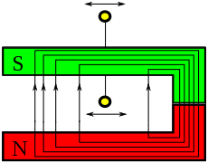
This principle is used in the transformer , the functional principle of which is sketched in the adjacent picture: If the battery circuit is closed in the left winding (primary winding), a changing magnetic field is created briefly in the iron core and an electrical voltage in the right winding (secondary winding) can be detected, for example, using a voltmeter or an incandescent lamp. If you reopen the battery circuit on the left side, an electrical voltage is generated again in the right winding. However, this has the opposite sign.

Heating a metal rod

If the iron core is electrically conductive, electrical currents can already be induced in the core, which heat the iron core (see picture "Heating a metal rod"). One tries to avoid this with transformers by using sheet metal cores, which offer a higher resistance to the current.

The generation of an electrical voltage can also be generated by moving the conductors. For example, an electrical alternating voltage can be tapped at the terminals of a conductor loop or a coil if the conductor loop is rotated in a magnetic field that is constant over time, as shown in the section Conductor loop in a magnetic field . According to the principle shown there (but a fundamentally improved arrangement), the generators used in power plants function to provide electrical energy in the power supply network. In the experiment shown, the direction of action can basically be reversed: If you apply an electrical alternating voltage to the terminals of the rotatably mounted conductor loop, the conductor loop rotates around its axis in the magnetic field ( synchronous motor ).

The movement of a conductor in a magnetic field can also be used to generate an electrical direct voltage . This is shown as an example in the section Induction by moving the conductor . If the conductor rod is moved along the rails, which are electrically connected to the conductor rod by a sliding contact or by wheels, a DC voltage can be measured on the voltmeter, which depends on the speed of the conductor rod, the magnetic flux density and the distance between the rails.

Faraday disc: When the aluminum disc is rotated, a direct voltage can be tapped from the voltmeter as a result of the unipolar induction . On the other hand, if you only turn the magnet, the voltage display remains at zero. If you turn the magnet and the aluminum disc at the same time, a voltage can again be measured.

Instead of a linear movement, the experiment can also be demonstrated with a rotary movement, as shown by the example of the Faraday disk (picture on the right). In the experiment shown, the aluminum disc takes over the function of the moving conductor rod from the experiment with the moving conductor rod in the magnetic field.

If the aluminum disc is rotated in a magnetic field, an electrical voltage can be detected between the sliding contact on the outer edge of the aluminum disc and the axis of rotation, with which, for example, an incandescent lamp can be operated. The voltage at the terminals depends on the strength of the magnetic flux density, the speed of rotation and the diameter of the disk. ${\ displaystyle \ omega _ {1}}$

To Faraday's astonishment, however, such a unipolar generator has unexpected properties that were discussed in the literature long after Faraday's discovery and led to a long-lasting controversy over the question of whether one could assign a speed to the magnetic field as it were to a material object and specifically whether the magnetic field rotates with the magnet. The main discovery was that, contrary to an obvious intuitive assumption, the voltage demonstrably does not depend on the relative movement between the permanent magnet and the aluminum disc. In the experiment shown, if you only turn the permanent magnet and let the aluminum disc rest ( ), no voltage can be observed despite the relative movement between the magnet and the conductor. If, on the other hand, both disks are rotated at the same speed ( ), tension is displayed, although the two disks do not move relative to one another. A voltage display can also be observed if the voltage is tapped directly from the permanent magnet, which is assumed to be electrically conductive, instead of the aluminum disc. ${\ displaystyle \ omega _ {1} = 0, \, \ omega _ {2} \ neq 0}$ ${\ displaystyle \ omega _ {1} = \ omega _ {2} \ neq 0}$

The principle is also reversible and allows magnetic disks through which current flows to spin, see homopolar motor .

Although the controversy surrounding this question can be resolved within the framework of Einstein's special theory of relativity and it has been proven that the relative speed between magnet and conductor is not important, the so-called hedgehog model of the magnetic field is still used in schools today, according to which the magnetic field lines like hedgehog spines attached to the magnet. According to the model, induction always occurs when the conductor "intersects" the field lines (relative movement between the conductor and the magnetic field). At the “Physics” seminar teacher conference in Dillingen in 2002, Hübel explicitly pointed out the difficulties associated with the hedgehog model and emphasized that the hedgehog model should not be misunderstood as a causal explanation of induction; on the contrary, it is not tenable and could lead to misconceptions.

Induction loop

A misconception that is just as common as the hedgehog spike model concerns the assumption that inductive processes can be explained using Kirchhoff's mesh equation . This means that the sum of all voltages in a circuit "once around the circle" always results in zero. From the law of induction, however, it can be concluded for static circuits that the sum of all voltages "once around" corresponds to the change in the magnetic flux that occurs in the area spanned by the circuit.

The picture opposite shows a conductor loop consisting of a good conductor (black line) and a resistor R, which is used to measure the voltage between terminals A and B. In the area within the rectangle (consisting of the conductor and the dashed connection between points A and B) there is a magnetic field, the time derivative of which is homogeneous and constant over time. ${\ displaystyle {\ frac {\ partial {\ vec {B}}} {\ partial t}}}$

If the voltage between terminals A and B is measured along a section through the air, the result is a value other than zero, which depends on the change in flux of the enclosed area: ${\ displaystyle u _ {\ mathrm {AB, Luft}} \ neq 0}$

If, on the other hand, the voltage between terminals A and B is measured along a section through the wire, the value is zero: because there is a vanishing E-field in the wire due to the low current flow and good conductivity, and the following applies: ${\ displaystyle u _ {\ mathrm {AB, wire}} = u_ {1} + u_ {2} + \ dotsb + u_ {15} = 0}$ ${\ displaystyle u_ {1} = u_ {2} = \ dotsb = u_ {15} = 0}$

The term "tension between two points" is no longer clear in the case of induction and must be supplemented by specifying the path (cf. vortex field ).

Induction in a conductor loop

General formulation of the law of induction for a conductor loop

The change over time in the magnetic flux enclosed by a conductor loop can be measured as a voltage at the ends of the conductor loop.

Although the general formulation of the law of induction does not require a conductor loop, as is customary in many introductory textbooks, induction on a conductor loop made of thin, highly conductive wire should first be considered. This allows a large number of technical applications such as motors and generators for three-phase and alternating current to be described and understood without the need to deal with the relativistic aspects of field theory or the application of the Lorentz transformation .

For the electrical voltage that can be measured between the two wire ends with a measuring device that is stationary or moving in the laboratory system (for example with an oscilloscope ) , the following conditions are met: ${\ displaystyle U}$

{\ displaystyle U = + {\ frac {{\ text {d}} \ Phi} {{\ text {d}} t}}.}

Here is the magnetic flux ${\ displaystyle \ Phi}$

{\ displaystyle \ Phi = \ int \ limits _ {{\ mathcal {A}} (t)} {\ vec {B}} \ cdot {\ text {d}} {\ vec {A}},}

which passes through any area delimited by the conductor loop, the supply lines to the measuring device and the lines in the measuring device . It can be shown that the calculation of the river does not depend on the shape of the surface, but only on its boundary. In the calculation it is also not necessary to distinguish whether the electrical voltage of the arrangement is generated by a change in the flux density or by a movement of the conductor. ${\ displaystyle {\ mathcal {A}} (t)}$

When specifying the sign in the equation , it should be noted that the sign depends both on the direction in which the measuring device is installed and on the orientation of the surface and must therefore always be read together with the associated circuit diagram. ${\ displaystyle U = {\ tfrac {{\ text {d}} \ Phi} {{\ text {d}} t}}}$

The surface orientation is indicated in the circuit diagram by the arrow drawn next to the surface element . The arrow next to the voltage specification in turn defines the installation direction of the measuring device. The voltage arrows (arrow points from top to bottom) mean that the red connection cable of the digital voltmeter is connected to the upper connection terminal and the black connection cable of the digital voltmeter is connected to the lower connection terminal . If the measuring device were to be turned around (voltage arrow from bottom to top) or if the surface orientation were to be reversed, the equation would have a negative sign. On the other hand, a positive sign would result if both the orientation of the stress arrow and the surface orientation were reversed. ${\ displaystyle {\ text {d}} {\ vec {A}}}$ ${\ displaystyle U}$

Example: induction by moving the conductor

If the conductor bar is moved, the measuring device shows the voltage . From the point of view of an observer resting in the laboratory system, there is an electrical field strength other than zero in the moving conductor rod. The field line image shows a pure source field, i. H. an electrostatic field. The two rails charge against each other like a capacitor. The vortex strength of the E-field is zero everywhere.

{\ displaystyle \ textstyle U = vLB_ {0}}

The measurement setup sketched in the adjacent picture consists of a static, electrically conductive rail arrangement over which a conductor bar slides at speed . The arrangement is located in a spatially and temporally constant magnetic field with the flux density , which is caused by a stationary permanent magnet or a stationary coil arrangement operated with direct current . The voltage between the two rails is measured with a voltmeter . ${\ displaystyle v}$ ${\ displaystyle {\ vec {B}} _ {0}}$

The voltage depends on the strength of the magnetic flux density , the speed and the rail spacing: ${\ displaystyle U}$ ${\ displaystyle B}$ ${\ displaystyle v}$ ${\ displaystyle L}$

{\ displaystyle U = L \ cdot B_ {0} \ cdot v}

This voltage can be understood with the help of the law of induction for a conductor loop formulated earlier. Since the magnetic field lines pierce the spanned surface perpendicularly, the magnetic flux can be calculated as

{\ displaystyle \ Phi = B_ {0} \ cdot A,}

where the area is a rectangular area with the area

{\ displaystyle A = L \ cdot x}

is.

The magnetic flux enclosed by the conductors is therefore:

{\ displaystyle \ Phi = B_ {0} \ cdot A = B_ {0} \ underbrace {Lx} _ {= A} = B_ {0} \ cdot L \ cdot x}

Since the speed is defined as

{\ displaystyle v = {\ frac {{\ text {d}} x} {{\ text {d}} t}},}

you can also write:

{\ displaystyle U = {\ frac {{\ text {d}} \ Phi} {{\ text {d}} t}} = B_ {0} \ cdot L \ cdot {\ frac {{\ text {d} } x} {{\ text {d}} t}} = B_ {0} \ cdot L \ cdot v}

In this case, one speaks of the so-called motion induction, since the voltage was created solely by the movement of the conductor and the change in the flux density over time did not play a role.

In the case of motion induction, the creation of the voltage can always be understood as a consequence of the Lorentz force on the conduction electrons present in the conductor rod. In the present example, the creation of the voltage is explained as follows:

The Lorentz force exerts a force on the electrons , which is the charge of an electron and the speed of the electron. ${\ displaystyle {\ vec {F}} _ {\ mathrm {L}} = q \ cdot \ left ({\ vec {v}} \ times {\ vec {B}} _ {0} \ right)}$ ${\ displaystyle q = -1 {,} 602 \ cdot 10 ^ {- 19} \ \ mathrm {C}}$ ${\ displaystyle {\ vec {v}}}$
The direction of the force can be traced with the UVW rule or the right-hand rule. In the drawing, the ladder is moved from left to right ( thumb of the right hand points to the right). The pale gray pattern in the background of the picture symbolizes field lines of the magnetic field that run away from the viewer perpendicular to the plane of the rail arrangement ( index finger points into the plane of the drawing). The middle finger points accordingly in the direction of the force that would be exerted on positive charge carriers ( middle finger points from the lower rail to the upper rail). As a result, negatively charged electrons are shifted towards the lower rail. ${\ displaystyle \ Rightarrow}$ ${\ displaystyle {\ vec {B}} _ {0}}$ ${\ displaystyle \ Rightarrow}$ ${\ displaystyle \ Rightarrow}$
Due to the Lorentz force, the electrons shift in such a way that there is a shortage of electrons on the upper rail and an excess of electrons on the lower rail.
The uneven charge distribution results in an electric field that counteracts the Lorentz force.
In the case of equilibrium, the Lorentz force and the Coulomb force are oppositely equal, and the following applies: ${\ displaystyle {\ vec {F}} _ {\ mathrm {L}}}$ ${\ displaystyle {\ vec {F}} _ {\ mathrm {C}}}$

{\ displaystyle {\ vec {E}} = - {\ vec {v}} \ times {\ vec {B}} _ {0}}

The electric field strength points in the direction of the lower rail and explains the terminal voltage that occurs.

Example: Induction by changing the flux density

If the flux density changes in the conductor circuit, the voltmeter shows a voltage.

A change in the magnetic flux can also be achieved by changing the magnetic flux density. In the example opposite, this is done by pushing a magnet coming from the left under the conductor loop. The representation was chosen in such a way that the same change in flux results as in the example " Induction by movement of the conductor ". As a result, there is also the same voltage at the terminals of the arrangement:

{\ displaystyle U = - {\ frac {{\ text {d}} \ Phi} {{\ text {d}} t}} = - B_ {0} \ cdot L {\ frac {{\ text {d} } x} {{\ text {d}} t}} = - B_ {0} \ cdot L \ cdot v}

Although the same flux change and the same voltage occur in both experiments, the two experiments are otherwise very different. This is especially true with regard to the electric field: In the example “ induction by movement of the conductor ” there is an electrostatic field, while in the example “ induction by flux density change ” there is an electric field with strong vortex components.

Technical applications

Historical induction apparatus from physics class

The law of induction is used in many ways in technology. What all examples have in common is that a change in the magnetic flux achieves a current-driving effect. This happens either by moving a conductor in a magnetic field (motion induction) or by changing the magnetic field:

Induction loop for vehicles to control traffic lights and barriers
Dynamic microphone
Dynamic (magnetic) pickup system for turntables
Pickups for electric string instruments (e.g. electric guitar and electric bass)
Sound head for scanning magnetic tapes
Generator = dynamo = alternator
RFID tag (e.g. ski pass)
Transcranial magnetic stimulation
Induction transmitter (also inductive pulse transmitter) as a speed sensor (e.g. in the automotive sector)
Induction hardening
Induction lamp
Induction transmitter
transformer
Induction loop system for the transmission of audio signals in hearing aids
Boost converter
betatron
Induction linear accelerator
Induction heating by eddy currents : induction furnace , induction hardening , the induction field , induction hob

Detecting the change in flow

If a voltage can be tapped at the terminals of a rigid conductor loop, this can always be traced back to a change in flux in the conductor loop, in accordance with the induction law for conductor loops.

When the conductor loop moves, a change in flux occurs.
When the conductor loop moves, a change in flux also occurs, but this is often not recognized.
The magnetic flux density in the legs of the horseshoe magnet is not constant.

Under the keyword "horseshoe paradox", Hübel points out that this change in flow remains hidden to the untrained eye in some cases and discusses the problems using various arrangements with horseshoe magnets, as they are typically used in school lessons (see adjacent pictures).

While the change in flow in the conductor loop in the first arrangement is usually easy to see for beginners, many learners fail in the second image. The learners concentrate on the air-filled area of the arrangement and do not take into account that the flux density increases continuously towards the pole of the permanent magnet only in the inner area, while it decreases significantly towards the poles in the magnet (see third picture).

Arrangement with rolling contacts - Hering experiment

A permanent magnet is moved into the conductor loop. Although there is a change in flux in the area under consideration, the voltmeter does not deflect.

The experiment on the Hering's Paradox , named after Carl Hering , shown on the right, shows that there is no deflection on the voltage measuring device, although there is a change in flow when viewed from a certain point of view.

Arrangement: A permanent magnet with ideal electrical conductivity is moved into a conductor loop at high speed . The upper and lower contact surfaces of the magnet are electrically conductively connected to the drawn conductor wires via fixed rollers. ${\ displaystyle v}$

Paradox: The apparent contradiction of the experiment to the law of induction can be resolved by a formal consideration. Form I and Form II with a stationary or convective (moving with the magnet) orbit curve lead to the (measured) result that no voltage is induced. The table gives an example of the terms that occur in Form II.

**Arrangement by C. Hering - Two variants of the stress calculation**
Induction law form II	${\ displaystyle \ textstyle \ partial {\ mathcal {A}}}$	${\ displaystyle \ textstyle {\ vec {u}}}$	${\ displaystyle \ textstyle \ int _ {\ mathrm {C} DAB} {\ vec {E}} \ cdot {\ text {d}} {\ vec {s}}}$	${\ displaystyle \ textstyle \ int _ {\ mathrm {B} C} {\ vec {E}} \ cdot {\ text {d}} {\ vec {s}}}$	${\ displaystyle \ textstyle \ int \ limits _ {\ mathrm {B} C} {\ vec {u}} \ times {\ vec {B}} \ cdot {\ text {d}} {\ vec {s}} }$	${\ displaystyle \ textstyle - {\ frac {\ text {d}} {{\ text {d}} t}} \ int \ limits _ {{\ mathcal {A}} (t)} {\ vec {B} } \ cdot {\ text {d}} {\ vec {A}}}$
${\ displaystyle \ textstyle \ oint \ limits _ {\ partial {\ mathcal {A}}} {({\ vec {E}} + {\ vec {u}} \ times {\ vec {B}}) \ cdot {\ text {d}} {\ vec {s}}} = - {\ frac {\ text {d}} {{\ text {d}} t}} \ int \ limits _ {\ mathcal {A}} {\ vec {B}} \ cdot {\ text {d}} {\ vec {A}} \ quad \ quad}$	resting	0	${\ displaystyle \ textstyle U}$	${\ displaystyle \ textstyle -vBL}$	0	${\ displaystyle \ textstyle -vBL}$
${\ displaystyle \ textstyle \ oint \ limits _ {\ partial {\ mathcal {A}} (t)} {({\ vec {E}} + {\ vec {u}} \ times {\ vec {B}} ) \ cdot {\ text {d}} {\ vec {s}}} = - {\ frac {\ text {d}} {{\ text {d}} t}} \ int \ limits _ {{\ mathcal {A}} (t)} {\ vec {B}} \ cdot {\ text {d}} {\ vec {A}} \ quad \ quad}$	convective	${\ displaystyle \ textstyle {\ vec {v}}}$	${\ displaystyle \ textstyle U}$	${\ displaystyle \ textstyle -vBL}$	${\ displaystyle \ textstyle + vBL}$	0

Compared to the high internal resistance of the voltmeter, the resistances on the stationary measuring line and the moving magnet are negligible. Therefore, in the resting part CDAB, an electric field strength can only exist in the voltmeter, so that there the contribution to the orbital integral is equal to (4th column of the table). The term in the 5th column comes from the fact that the moving magnetized body appears to be electrically polarized in the laboratory system. The term indicates the corresponding electrical voltage. The transformation relationship between electric field strength and magnetic flux density according to Lorentz also leads to the same result . The movement of the edge line is included in the magnetic shrinkage in the column on the far right. With a moving section BC, the flow remains constant. With the specified terms, stationary or moving edge lines lead to the (also measured) result . ${\ displaystyle \ textstyle {\ vec {E}}}$ ${\ displaystyle \ textstyle U}$ ${\ displaystyle \ textstyle -vLB}$ ${\ displaystyle \ textstyle {\ vec {E}} '= {\ vec {E}} + {\ vec {v}} \ times {\ vec {B}}}$ ${\ displaystyle \ textstyle {\ vec {E}} '= 0}$ ${\ displaystyle \ textstyle U = 0}$

General law of induction in differential form and in integral form

The law of electromagnetic induction, or induction law for short, describes the relationship between electric and magnetic fields. It says that when the magnetic flux changes through a surface at the edge of this surface, a ring stress is created. In particularly frequently used formulations, the law of induction is described by showing the edge line of the surface as an interrupted conductor loop, at the open ends of which the voltage can be measured.

The description, which is useful for understanding, is divided into two possible forms of representation:

The integral form or global form of the law of induction: This describes the global properties of a spatially extended field area (via the integration path).
The differential form or local form of the law of induction: The properties of individual local field points are described in the form of densities. The volumes of the global form tend towards zero, and the field strengths that arise are differentiated.

Both forms of representation describe the same facts. Depending on the specific application and problem, it can make sense to use one or the other form.

When applying the law of induction, it should be noted that all quantities occurring in the equations, i.e. H. the electric field strength , the magnetic flux density , the oriented surface , the contour line of this surface and the local speed of a point on the contour line can be described from any reference system ( inertial system ) which is the same for all quantities . ${\ displaystyle {\ vec {E}}}$ ${\ displaystyle {\ vec {B}}}$ ${\ displaystyle {\ mathcal {A}}}$ ${\ displaystyle \ partial {\ mathcal {A}}}$ ${\ displaystyle {\ vec {u}}}$

If the contour line leads through matter, the following must also be observed:

The contour line is an imaginary line. Since it has no physical equivalent, a possible temporal movement of the contour line has basically no influence on the physical processes taking place. In particular, a movement of the contour line does not change the field sizes and . In the integral form I, the movement of the contour line is therefore not taken into account at all. In integral form II, the movement of the imaginary contour line affects both sides of the equation to the same extent, so that when calculating, for example, an electrical voltage with integral form I, the same result is obtained as when calculating the same voltage using integral form II. ${\ displaystyle \ partial {\ mathcal {A}}}$ ${\ displaystyle {\ vec {E}}}$ ${\ displaystyle {\ vec {B}}}$
In principle, the speed of the contour line may deviate from the speed of the bodies used in the experiment (e.g. conductor loop, magnets). The speed of the contour line in relation to the observer is indicated in the context of the article with , while the speed of objects is described with the letter . ${\ displaystyle {\ vec {u}}}$ ${\ displaystyle {\ vec {v}}}$
In contrast to the movement of the contour line, the speed of the body generally has an influence on the physical processes that take place. This applies in particular to the field sizes and which the respective observer measures. ${\ displaystyle {\ vec {E}}}$ ${\ displaystyle {\ vec {B}}}$

Law of induction in differential form

The law of induction in differential form reads:

{\ displaystyle \ operatorname {red} {\ vec {E}} = - {\ dot {\ vec {B}}}}

The presence of electrical eddies or a time-varying magnetic flux density is the essential characteristic of induction. In electric fields without induction (e.g. in the field of immobile charges) there are no closed field lines of the electric field strength , and the orbital integral of the electric field strength always results in zero. ${\ displaystyle E}$

The law of induction finds its main application in differential form, on the one hand, in theoretical derivations and in numerical field computation, and, on the other hand (but less often) in the analytical computation of specific technical questions.

As shown in Einstein's first work on special relativity, the Maxwell equations are in differential form in agreement with special relativity. A derivation for this that has been adapted to today's linguistic usage can be found in Simonyi's textbook, which is now out of print.

Transition from the differential form to the integral form

The relationship between the integral form and the differential form can be described mathematically using Stokes' theorem. The global vortex and source strengths are converted into local, discrete vortex or source densities, which are assigned to individual spatial points (points of a vector field ).

The starting point is the law of induction in differential form:

{\ displaystyle \ operatorname {rot} {\ vec {E}} = - {\ frac {\ partial {\ vec {B}}} {\ partial t}}}

For the conversion into the integral form, the Stokes theorem is used, which for obvious reasons is formulated with the variable : ${\ displaystyle {\ vec {E}}}$

{\ displaystyle \ oint \ limits _ {\ partial {\ mathcal {A}}} {\ vec {E}} \, {\ text {d}} {\ vec {s}} = \ int \ limits _ {\ mathcal {A}} \ operatorname {red} {\ vec {E}} \, {\ text {d}} {\ vec {A}}}

If one replaces the vector field in the right term of Stokes' law according to the law of induction in differential form by the term , then we get: ${\ displaystyle {\ vec {E}}}$ ${\ displaystyle - {\ tfrac {\ partial {\ vec {B}}} {\ partial t}}}$

{\ displaystyle \ oint \ limits _ {\ partial {\ mathcal {A}}} {\ vec {E}} \, {\ text {d}} {\ vec {s}} = - \ int \ limits _ { \ mathcal {A}} {\ frac {\ partial {\ vec {B}}} {\ partial t}} \, {\ text {d}} {\ vec {A}}}

This is a possible general form of the law of induction in integral form, which, contrary to many statements to the contrary, can be used for contour lines in bodies at rest as well as in moving bodies.

To get a formulation that contains the magnetic flux , add the term on both sides of the equation . This results in: ${\ displaystyle \ Phi = \ int \ limits _ {\ mathcal {A}} {\ vec {B}} \, {\ text {d}} {\ vec {A}}}$ ${\ displaystyle \ oint \ limits _ {\ partial {\ mathcal {A}}} ({\ vec {u}} \ times {\ vec {B}}) \, {\ text {d}} {\ vec { s}}}$

{\ displaystyle \ oint \ limits _ {\ partial {\ mathcal {A}}} \ left ({\ vec {E}} + {\ vec {u}} \ times {\ vec {B}} \ right) \ , {\ text {d}} {\ vec {s}} = - \ int \ limits _ {\ mathcal {A}} {\ frac {\ partial {\ vec {B}}} {\ partial t}} \ , {\ text {d}} {\ vec {A}} + \ oint \ limits _ {\ partial {\ mathcal {A}}} ({\ vec {u}} \ times {\ vec {B}}) \, {\ text {d}} {\ vec {s}}}

The right part of the equation corresponds to the negative temporal change of the magnetic flux, so that the law of induction can also be noted in integral form with full general validity as follows: ${\ displaystyle \ operatorname {div} {\ vec {B}} = 0}$

{\ displaystyle \ oint \ limits _ {\ partial {\ mathcal {A}}} \ left ({\ vec {E}} + {\ vec {u}} \ times {\ vec {B}} \ right) \ , {\ text {d}} {\ vec {s}} = - {\ frac {\ text {d}} {{\ text {d}} t}} \ int \ limits _ {\ mathcal {A}} {\ vec {B}} \, {\ text {d}} {\ vec {A}}}

In many textbooks, these relationships are unfortunately not properly noted, which can be seen from the fact that the term noted on the left side of the equation is missing. The error has been corrected in the new edition. The law of induction, on the other hand, is correctly noted by Fließbach, for example. ${\ displaystyle {\ vec {u}} \ times {\ vec {B}}}$

The mistake is probably that the missing term is mistakenly added to the electric field strength. (Some authors also speak of an effective electric field strength in this context .) As a consequence, omitting the term means that the quantity is used inconsistently and has a different meaning depending on the context. ${\ displaystyle {\ vec {u}} \ times {\ vec {B}}}$ ${\ displaystyle E}$

Law of induction in integral form

The voltage between the two points A and B along the path shown is the sum of the products of the electric field strength and the length of the path

{\ displaystyle {\ vec {E}} \ cdot {\ text {d}} {\ vec {r}}}

{\ displaystyle {\ vec {E}}}

{\ displaystyle {\ text {d}} {\ vec {r}}.}

In the following section the first integral form of the law of induction is considered:

{\ displaystyle \ oint \ limits _ {\ partial {\ mathcal {A}}} {\ vec {E}} \, \ mathrm {d} {\ vec {s}} = - \ int \ limits _ {\ mathcal {A}} {\ frac {\ partial {\ vec {B}}} {\ partial t}} \, \ mathrm {d} {\ vec {A}}}

According to the mathematical formulation of the integral, the area is considered at a constant point in time and its change over time is not taken into account. ${\ displaystyle {\ mathcal {A}}}$

With regard to the concept of the induced voltage - the integral over the electric field strength - the connection line drawn in the adjacent picture between points A and B in an electric field is first considered.

The voltage between points A and B (“outer pole” of a “socket”) can be calculated approximately by dividing the path into many small path elements . Since, due to the short length, an approximately constant electric field strength along such a section of the path can be assumed, the value for the partial voltage along a path element in the interior results ${\ displaystyle {\ text {d}} {\ vec {r}}}$

{\ displaystyle {\ text {d}} U \ approx + {\ vec {E}} (x, y, z) \ cdot {\ text {d}} {\ vec {r}} = {+ {E} _ {\ text {tan}}} \, {\ text {d}} r.}

The total tension between the two points is thus obtained

{\ displaystyle \ Delta U \ approx + {\ vec {E}} ({{x} _ {1}}, {{y} _ {1}}, {{z} _ {1}}) \ cdot { \ text {d}} {{\ vec {r}} _ {1}} + {\ vec {E}} ({{x} _ {2}}, {{y} _ {2}}, {{ z} _ {2}}) \ cdot {\ text {d}} {{\ vec {r}} _ {2}} + \ dotsb + {\ vec {E}} ({{x} _ {n} }, {{y} _ {n}}, {{z} _ {n}}) \ cdot {\ text {d}} {{\ vec {r}} _ {n}}.}

The exact representation is defined using an integral. This can be imagined as a limit value for an infinite number of path sections with an infinitely small length . For the calculation one defines i. A. a function that is dependent on a parameter and describes the points along the route in the area ( i.e. in the interior in the direction of the arrow). The tension between the two points can then be formally recorded using a curve integral: ${\ displaystyle \ left | {\ text {d}} {\ vec {r}} \ right | \ to 0}$ ${\ displaystyle \ xi}$ ${\ displaystyle {\ vec {r}} (\ xi)}$ ${\ displaystyle \ xi = 0 \ dots 1}$

{\ displaystyle \ Delta U = \ int _ {\ xi = 0} ^ {1} {{\ vec {E}} (} {\ vec {r}}) \ cdot {\ frac {\ partial {\ vec { r}} (\ xi)} {\ partial \ xi}} {\ text {d}} \ xi =: \ int _ {A} ^ {B} {\ vec {E}} \ cdot {\ text {d }} {\ vec {r}} \ ,,}

calculated in the direction of the arrow

If the point is now allowed to move along the contour of a complete circuit until it has circled the enclosed area exactly once and is again identical to the starting point , the total value is the circuit voltage induced in the closed conductor loop : ${\ displaystyle C = \ partial {\ mathcal {A}}}$ ${\ displaystyle (B = A),}$ ${\ displaystyle U _ {\ text {ind}}}$

{\ displaystyle U _ {\ text {ind}} = \ oint _ {C} E _ {\ text {tan}} {\ text {d}} r = \ oint _ {C} {\ vec {E}} \ cdot {\ text {d}} {\ vec {r}}}

With regard to the sign, it must be taken into account that the contour surrounds the surface in the sense of the right-hand rule.

The third expression of the above equations is the vector representation of the tangential field strength component with the help of the scalar product , which is equivalent to the second expression , and the two integrals are so-called ring integrals , which are always used when (as here) is integrated along a closed path, in this case along the contour of the conductor loop ${\ displaystyle C.}$

With a non-moving conductor loop, the induced voltage can be measured approximately as a voltage drop with a voltage measuring device if a conductor loop is attached along the closed line and it is cut at one point. Since there is almost no electrical voltage across the conductor wire, all of the induced voltage lies between the terminals.

Relativistic aspects

In measuring systems with moving components, relativistic effects occur even at low speeds . This fundamental fact becomes clear through a simple thought experiment: ${\ displaystyle v \ ll c}$

An observer who observes a charge (not moving relative to him) will measure an electric field, but no magnetic field due to the lack of current flow.
If, on the other hand, the observer moves towards or away from the charge, he will on the one hand notice that the electric field changes due to the movement. This means that the observer measures a different field at the same distance from the charge but at a different speed relative to the charge . On the other hand, the observer also interprets the charge as a current moving away from or towards him. The observer will also see a magnetic field in addition to the electric field. ${\ displaystyle E}$

In order to avoid misunderstandings when measuring with moving components, it is essential to specify the reference system relative to which the observations are described. It is also necessary to convert quantities that are measured in a reference system other than the one on which they are based, using the Lorentz transformation .

The application of the Lorentz transformation is particularly important when considering electrical field strengths. Contrary to popular belief, this is necessary at speeds far below the speed of light (for example a few mm / s) and is important in practically all experiments with moving conductors.

Experiment with a moving ladder rod in a field that is constant over time

{\ displaystyle B}

To explain this, we look again at the moving conductor bar in the field that is constant over time . ${\ displaystyle B}$

Since the conductor loop is open, the current driving force on a charge is ${\ displaystyle {\ vec {F}}}$ ${\ displaystyle q}$

{\ displaystyle {\ vec {F}} = q \ cdot ({\ vec {E}} + {\ vec {v}} \ times {\ vec {B}} _ {0}) = 0.}

From the perspective of an observer in the laboratory system, the field strength is thus obtained in the conductor rod moving with the speed ${\ displaystyle {\ vec {v}}}$

{\ displaystyle {\ vec {E}} = - {\ vec {v}} \ times {\ vec {B}} _ {0} \ neq 0,}

while in the area of the stationary conductor with a field strength of ${\ displaystyle {\ vec {v}} = 0}$

{\ displaystyle {\ vec {E}} = 0}

prevails.

The differences in the field strength between the moving and stationary conductor sections result directly from the Lorentz transformation for the electrical field strength: An observer who moves with the moving conductor rod will have an (intrinsic) field strength of within the conductor rod

{\ displaystyle {\ vec {E}} '= {\ vec {0}}}

measure up. If the (deleted) self-field strength is inserted into the appropriate transformation equation, the result for the corresponding variable in the laboratory system is:

{\ displaystyle {\ vec {E}} '= \ gamma \ left ({\ vec {E}} + {\ vec {v}} \ times {\ vec {B}} _ {0} \ right) + ( 1- \ gamma) {\ frac {{\ vec {E}} \ cdot {\ vec {v}}} {{v} ^ {2}}} {\ vec {v}} = {\ vec {0} }}

Because of that , the entire right term is omitted and with it the relevance of the factor , which can be “divided into zero”, so to speak. As expected, this results in the value for the electrical field strength from the perspective of the laboratory system ${\ displaystyle {\ vec {v}} \ perp {\ vec {E}}}$ ${\ displaystyle \ gamma}$

{\ displaystyle {\ vec {E}} = - {\ vec {v}} \ times {\ vec {B}}.}

With the help of this experiment one can demonstrate relativity theory with simple lecture experiments. Since the experiment mentioned is shown in many representations as an example of electromagnetic induction, it should be expressly confirmed that the terminal voltage cannot be traced back to eddies of the electric field, because there are none. As the field line picture shows, there is a pure potential field. These show from positive charges on the surface of the upper rail to negative charges on the surface of the lower rails. In this sense, the physical process that takes place in this experiment can be compared to the charging of a capacitor. ${\ displaystyle \ operatorname {rot} {\ vec {E}} = {\ dot {\ vec {B}}} = 0}$

Considerations of special questions

Induction example: moving conductor rod in a magnetic field (with current flow)

If the conductor loop is closed and the rod moves in the magnetic field, there is a current flow in the circuit.

In a modification of the example of a “moving conductor bar in a homogeneous magnetic field” discussed above, a circuit with finite resistance is considered here, so that a current flow occurs when the conductor bar moves in the magnetic field. The following applies to the amperage:

{\ displaystyle I = {\ frac {U} {R}} = {\ frac {\ frac {{\ text {d}} \ Phi} {{\ text {d}} t}} {R}}}

The entire change in flux in the conductor loop is considered here. However, since the inductance for a conductor arrangement as here can be approximated, the current-dependent magnetic flux and the associated change in flux are also negligible. The induced current strength is thus: ${\ displaystyle L _ {\ Phi} \ approx 0}$ ${\ displaystyle \ Phi _ {L} = L _ {\ Phi} I \ approx 0}$ ${\ displaystyle {\ tfrac {{\ text {d}} \ Phi _ {L}} {{\ text {d}} t}} = L _ {\ Phi} {\ tfrac {{\ text {d}} I } {{\ text {d}} t}} \ approx 0}$

{\ displaystyle I = {\ frac {vLB_ {0}} {R}}}

If the ladder bar is moved at the constant speed , mechanical work is carried out. The force is the Lorentz force on a current-carrying conductor of the length in the magnetic field of the flux density : ${\ displaystyle v}$ ${\ displaystyle L}$ ${\ displaystyle B_ {0}}$

{\ displaystyle {\ vec {F}} = I {\ vec {L}} \ times {\ vec {B}} _ {0},}

here:

{\ displaystyle F = ILB_ {0}}

For the electrical power , which is converted in the resistor, applies and for the mechanical power of such a uniform movement , after one has inserted the corresponding quantities from above. So mechanical work is converted into electrical work. ${\ displaystyle P = UI}$ ${\ displaystyle P = vF = vILB_ {0} = {\ frac {U} {LB_ {0}}} ILB_ {0} = UI}$

Induction example: conductor loop in a magnetic field

A conductor loop rotates in the magnetic field.

If a conductor loop rotates at angular velocity in a magnetic field that is constant over time, viewed from the laboratory system, the magnetic flux density changes constantly from the point of view of the conductor loop, and there is a changed magnetic flux through the conductor loop. ${\ displaystyle \ omega = 2 \ pi f}$

The voltage measured at the terminals in the rotating system can be calculated as follows:

The flat surface bordered by the conductor loop has the area .

{\ displaystyle A = l_ {1} l_ {2}}

The magnetic flux density constantly changes its magnitude and direction in the co-ordinate system of the moving observer. If one assumes that the image shows the area at the point in time , then the proportion of the flux density occurring perpendicular to the area is .

{\ displaystyle t = 0}

{\ displaystyle B _ {\ mathrm {perpendicular}} (t) = \ cos (2 \ pi ft) B}

The magnetic flux penetrating through the surface is accordingly .

{\ displaystyle A}

{\ displaystyle \ Phi (t) = BA \ cos (2 \ pi ft)}

For the voltage it follows with the help of the chain rule : ${\ displaystyle U}$

{\ displaystyle U = {\ frac {{\ text {d}} \ Phi} {{\ text {d}} t}} = BA (-2 \ pi f) \ sin (2 \ pi ft)}

Induction example: Induction with an electrical coil with several turns

Area of a coil with three turns

The law of induction is also applicable to electrical coils with several turns. The area required to calculate the magnetic flux is illustrated in the adjacent picture. The law of induction in its general form therefore does not require a factor for the number of turns of the coil, even if the coil wire in a specific case revolves around a cylinder several times. ${\ displaystyle N}$

In most of the publications on electromagnetic induction in electrical coils, the number of turns factor is introduced for the sake of simplicity , and the law of induction is given in the form ${\ displaystyle N}$

{\ displaystyle U = {\ frac {{\ text {d}} \ Psi} {{\ text {d}} t}} \ approx N {\ frac {{\ text {d}} \ Phi _ {\ text {w}}} {{\ text {d}} t}}}

specified. Here, the flux through a surface bordered by the coil wire and the connections denotes the magnetic flux enclosed by a single turn, and is the measured voltage. ${\ displaystyle \ Psi}$ ${\ displaystyle \ Phi _ {\ text {w}}}$ ${\ displaystyle U}$

Formulation variant: Ohm's law for moving conductors

The relationships in motion induction can also be grasped relatively easily using Ohm's law for moving conductors. In contrast to a stationary conductor, in which only the electric field strength drives the current, the full Lorentz force acts on the charges in a moving conductor

{\ displaystyle {\ vec {F}} _ {\ mathrm {L}} = q ({\ vec {E}} + {\ vec {v}} \ times {\ vec {B}}).}

For non-relativistic velocities , the Lorentz force measured in the stationary reference system is the same as the force experienced by the charge in the moving system. ${\ displaystyle v \ ll c}$

For moving materials to which Ohm's law applies, the specific conductivity can be given by the equation ${\ displaystyle \ kappa}$

{\ displaystyle {\ vec {J}} = \ kappa ({\ vec {E}} + {\ vec {v}} \ times {\ vec {B}})}

be defined with the electric field strength , the speed of the respective conductor element and the magnetic flux density . Ohm's law then reads as in the case of immobile materials ${\ displaystyle {\ vec {E}}}$ ${\ displaystyle {\ vec {v}}}$ ${\ displaystyle {\ vec {B}}}$

{\ displaystyle {\ begin {aligned} \ kappa = {\ text {constant}} \ end {aligned}}.}

Formulation variant: form integrated in time, tension-time area

The hatched area represents an exemplary voltage-time area over the duration of a quarter period of the sinusoidal oscillation (100% at 325 V peak voltage).

By integrating over time, the law of induction for conductor loops can be transformed as follows:

{\ displaystyle \ Phi _ {\ text {w}} (t) = \ Phi _ {\ text {w}} (0) + {\ frac {1} {N}} \ cdot \ int \ limits _ {0 } ^ {t} U _ {\ mathrm {i}} (\ tau) \, {\ text {d}} \ tau}

This relationship describes the flow curve as an integral function of the voltage curve.

If you consider the process in a time interval of up to with a constant area through which the magnetic flux passes - the time interval can, for example, extend over a half period of an alternating voltage - then it follows for the flux that then results ${\ displaystyle 0}$ ${\ displaystyle T}$

{\ displaystyle \ Phi _ {\ mathrm {w}} (T) - \ Phi _ {\ mathrm {w}} (0) = {\ frac {1} {N}} \ cdot \ int _ {0} ^ {T} U _ {\ mathrm {i}} (\ tau) \, \ mathrm {d} \ tau.}

In the case that the magnetic flux through a conductor loop or a flux change in this, as they are by applying a voltage after the given time, this means always stops there from the voltage time integral within the indicated limits to be caused and this also must correspond to . The voltage relevant for this is the induced voltage in each case . This corresponds to the applied voltage minus ohmic voltage drops insofar as these cannot be neglected. ${\ displaystyle \ Phi _ {\ mathrm {w}} (0) = 0}$ ${\ displaystyle T}$ ${\ displaystyle 0}$ ${\ displaystyle T}$ ${\ displaystyle U _ {\ mathrm {i}}}$ ${\ displaystyle (I \ cdot R),}$

The stress-time integral can also be illustrated as the area between the stress graph and the time axis over the interval, which is why it is sometimes also referred to as the stress- time area or stress-time sum , in mostly older literature, based on the term impulse, also as a surge. The reason for this is the fact that, in terms of measurement technology, the integration of induced voltage pulses was previously carried out by means of ballistic galvanometers , see also illustration of the magnetic flux of force . ${\ displaystyle [0; T],}$

Example for 50 Hz at : Determined graphically by counting the small squares, you get the result of approx. 1.05 volt-seconds for the picture on the top right, for a sinusoidal half-oscillation consequently 2.1 volt-seconds. This is the voltage-time area that the induction in the iron core of a transformer transports from one end of the hysteresis curve to the other end. If a transformer is designed to match the 230 V at 50 Hz, the induction runs in continuous operation mainly in the vertical area of the hysteresis curve. Higher voltage or lower frequency leads to an overdrive of the hysteresis curve in the horizontally running areas, to core saturation, which can then also be clearly observed in practice through the increase in the magnetizing current. ${\ displaystyle U _ {\ text {eff}} = 230 \, {\ text {V}}}$

A widely practiced measuring principle for the magnetic flux can serve as a further example: Here the flux to be measured is recorded by a measuring coil and the voltage on the coil is sent to an integrator, which immediately displays the flux at its output.

Formulation variant: flow rule

The flow rule formulates the law of induction in integral form for the special case of a conductor loop: It applies to closed circular paths that run entirely in electrically conductive (also moving) material in the (also time and location-variable) magnetic field, preferably in conductor loops with a small cross-section. In the case of moving conductor loops, the specified orbital curve must develop continuously and convectively (see below) without interruptions. The speeds in the arrangement must be significantly lower than the speed of light. ${\ displaystyle U_ {i} = - {\ dot {\ Phi}}}$

Derivation: The circulation path in the induction law Form II can largely be freely used. In the approach leading to the flow rule, the local material velocity is given to all elements of the circulation path (convective line elements, ). The following applies: ${\ displaystyle {\ text {d}} {\ vec {s}}}$ ${\ displaystyle {\ vec {v}}}$ ${\ displaystyle {\ vec {u}} = {\ vec {v}}}$

{\ displaystyle \ oint \ limits _ {\ partial {\ mathcal {A}} (t)} {({\ vec {E}} + {\ vec {v}} \ times {\ vec {B}}) \ cdot {\ text {d}} {\ vec {s}}} = - {\ frac {\ text {d}} {{\ text {d}} t}} \ int \ limits _ {{\ mathcal {A }} (t)} {\ vec {B}} \ cdot {\ text {d}} {\ vec {A}}}

.

According to Lorentz's transformation equations, the integrand of the left term is equal to the electric field strength in the rest frame of each line element, so that too ${\ displaystyle {\ vec {E}} '}$

{\ displaystyle \ oint \ limits _ {\ partial {\ mathcal {A}} (t)} {{\ vec {E}} '\ cdot {\ text {d}} {\ vec {s}}} = - {\ frac {\ text {d}} {{\ text {d}} t}} \ int \ limits _ {{\ mathcal {A}} (t)} {\ vec {B}} (t) \ cdot {\ text {d}} {\ vec {A}} \ quad (*)}

or shorter

{\ displaystyle U_ {i} = - {\ dot {\ Phi}}}

can be written. The last two equivalent equations are initially tailored forms of the law of induction for the above-mentioned conditions. The last equation is known as the flow rule when applied to an unbranched circuit. The electromagnetic quantity that drives the current , known as induced voltage - by definition a ring voltage - proves to be equal in value to magnetic fading . A voltmeter installed somewhere in the conductor circuit, the internal resistance of which is large compared to the resistance of the rest of the circuit, shows the value of . ${\ displaystyle U_ {i}}$ ${\ displaystyle - {\ dot {\ Phi}}}$ ${\ displaystyle U_ {i}}$

That the magnetic loss (in Eq. ( ) Of the right term) can drive an electric current through the electrical resistance in the conductor loop, in the form illustrated the link Terms: There the charge-related work which the Lorentz force performed at the charge at a loop circulation. The convenience of using the flow rule lies in the fact that the current-driving induced voltage in a stationary or moving conductor loop can be determined solely from the magnetic field: The electric field strength in the laboratory system and that in the rest system of the line elements do not appear in the formula. ${\ displaystyle - {\ dot {\ Phi}}}$ ${\ displaystyle *}$ ${\ displaystyle U_ {i}}$ ${\ displaystyle {\ vec {E}}}$ ${\ displaystyle {\ vec {E}} '}$

The windings of transformers, electric motors and generators for power generation are conductor loops in the sense of the flux rule.

Example breathing conductor loop

Conductor loop with a time-varying radius (breathing) in a time-varying magnetic field

The circular (imaginary elastic) conductor loop sketched on the right with a time-varying radius is located in a homogeneous, time-dependent magnetic field . The conductor cross-section and the electrical conductivity can vary along the circumference. The time derivative of the radius turns out to be the local, radially directed speed of the ring elements. The loop plane is normal to the axis and remains parallel to itself. In the sketch, the arrows indicate the radial, peripheral and axial unit vectors , and also the reference directions for the scalar quantities in question. All field sizes given below are time-dependent, which the notation does not repeat every time. ${\ displaystyle r (t)}$ ${\ displaystyle {\ vec {B}} = B (t) {\ vec {e}} _ {z}}$ ${\ displaystyle A}$ ${\ displaystyle \ kappa}$ ${\ displaystyle {\ dot {r}} = v}$ ${\ displaystyle r}$ ${\ displaystyle v}$ ${\ displaystyle z}$ ${\ displaystyle {\ vec {e}} _ {\ rho}}$ ${\ displaystyle {\ vec {e}} _ {\ varphi}}$ ${\ displaystyle {\ vec {e}} _ {z}}$

The voltage induced in the loop drives an electric current along with it . Its field-generating effect is assumed to be negligible or already included. ${\ displaystyle U_ {i} = - {\ dot {\ Phi}} = - {\ tfrac {\ text {d}} {{\ text {d}} t}} (B {\ vec {e}} _ {z} \ cdot \ pi r ^ {2} {\ vec {e}} _ {z}) = - {\ dot {B}} \ pi r ^ {2} -B \ pi 2rv}$ ${\ displaystyle I = U_ {i} / R}$ ${\ displaystyle R = \ oint _ {\ partial {\ mathcal {A}}} {\ tfrac {{\ text {d}} s} {\ kappa A}}}$ ${\ displaystyle {\ vec {B}} (t)}$

The electric field quantities that are eliminated from the flow rule are given below for information purposes only. For the current density and the electric field strength in the rest system of the ring elements applies or . Obtained with the electric field strength in the rest of the loop center the result . The last equation follows with . In the event that the conductor cross-section and the conductivity at the circumference are constant, the rotational symmetry of the arrangement is also reflected in the field sizes. The field coordinates and are then obtained . ${\ displaystyle {\ vec {S}} = {\ vec {e}} _ {\ varphi} I / A}$ ${\ displaystyle {\ vec {E}} '= {\ vec {S}} / \ kappa}$ ${\ displaystyle {\ vec {E}} = {\ vec {E}} '- {\ vec {v}} \ times {\ vec {B}}}$ ${\ displaystyle {\ vec {E}} = (S / \ kappa + vB) {\ vec {e}} _ {\ varphi}}$ ${\ displaystyle {\ vec {v}} \ times {\ vec {B}} = v {\ vec {e}} _ {\ rho} \ times B {\ vec {e}} _ {z} = - Bv {\ vec {e}} _ {\ varphi}}$ ${\ displaystyle E '= U_ {i} / (2 \ pi r) = - {\ dot {B}} r / 2-Bv}$ ${\ displaystyle E = - {\ dot {B}} r / 2}$

Example tension in the vortex field

Ambiguity of the electrical voltage in a time-varying magnetic field. The signs + and - are engravings on the voltmeter housings.

The arrangement on the right illustrates, based on the flow rule, that the voltage tapped on a conductor loop (linked to a time-varying magnetic field) depends on the placement of the measuring lines. The tension between two points is then no longer a clear concept.

In the measurement setup, two voltage meters with the same polarity contact points A and B of a conductive frame in the form of a regular pentagon. Its ohmic resistance is . In the conductor loop, the induced voltage drives the current . No flow is linked to the circulation path through the measuring device 1 and the frame side AB. The voltmeter 1 shows the value according to the voltage equation . With the alternative circuit A – C – B – Voltmeter1 for calculating the time-varying magnetic flux is concatenated, so that the voltage equation applies. From this it follows again . ${\ displaystyle 5R}$ ${\ displaystyle U_ {i} = - {\ dot {\ Phi}}}$ ${\ displaystyle I = U_ {i} / (5R)}$ ${\ displaystyle -U_ {1} -RI = 0}$ ${\ displaystyle U_ {1} = - U_ {i} / 5}$ ${\ displaystyle U_ {1}}$ ${\ displaystyle \ Phi (t)}$ ${\ displaystyle 4RI-U_ {1} = U_ {i} \, (= - {\ dot {\ Phi}})}$ ${\ displaystyle RI = U_ {i} / 5}$ ${\ displaystyle U_ {1} = - U_ {i} / 5}$

Corresponding equations apply to voltmeter 2: The one with no chained flow along A – Voltmeter2 – B – C – A is . The alternative circuit A – Voltmeter2 – B – A with the voltage equation is linked to the flux . Calculate from both circuits . ${\ displaystyle U_ {2} -4RI = 0}$ ${\ displaystyle U_ {2} + RI = U_ {i}}$ ${\ displaystyle \ Phi (t)}$ ${\ displaystyle U_ {2} = (4/5) U_ {i}}$

The (comparison) cycle that does not go through any frame part only via the two tension meters provides the equation that is satisfied with the above terms for and . ${\ displaystyle -U_ {1} + U_ {2} = U_ {i}}$ ${\ displaystyle U_ {1}}$ ${\ displaystyle U_ {2}}$

Self induction

literature

Karl Küpfmüller , Gerhard Kohn: Theoretical electrical engineering and electronics . 14th edition. Springer, 1993, ISBN 3-540-56500-0 .
Adolf J. Schwab : Conceptual world of field theory. Electromagnetic fields, Maxwell's equations, gradient, rotation, divergence . 6th edition. Springer, 2002, ISBN 3-540-42018-5 .
Heinrich Frohne , Karl-Heinz Locher, Hans Müller, Thomas Marienhausen, Dieter Schwarzenau: Moeller basics of electrical engineering (studies) . 22nd edition. Vieweg + Teubner Verlag, Springer Fachmedien, Berlin / Offenbach 2011, ISBN 978-3-8348-0898-1 , p. 252 ff .

Web links

Electromagnetic induction. Induction at student level at LeiFi Physik.
Helmut Haase: voltage induction and flow rule. ( Memento of August 29, 2014 in the Internet Archive ). (PDF; 21 pages; 2.5 MB).
Video: Induction in static conductors . Institute for Scientific Film (IWF) 2004, made available by the Technical Information Library (TIB), doi : 10.3203 / IWF / C-14868 .
Video: Induction in moving conductors . Institute for Scientific Film (IWF) 2004, made available by the Technical Information Library (TIB), doi : 10.3203 / IWF / C-14869 .

References and footnotes

↑ ^a ^b Douglas C. Giancoli: Physics: Principles with Applications . 5th edition. 1998, p. 623-624 .

↑ Fawwaz Ulaby: Fundamentals of applied electromagnetics . 5th edition. Pearson Prentice Hall, 2007, ISBN 978-0-13-241326-8 , pp. 255 .

↑ Joseph Henry. (No longer available online.) In: Distinguished Members Gallery, National Academy of Sciences. Archived from the original on December 13, 2013 ; Retrieved November 30, 2006 .

↑ Bence Jones: The Life And Letters Of Faraday . Volume II, 2008, ISBN 978-1-4437-1530-0 ( limited preview in Google Book Search).

↑ Leslie Pearce Williams : Michael Faraday. A biography . Chapman and Hall, London 1965, p. 182-183 (English).

↑ Leslie Pearce Williams: Michael Faraday: A biography . Chapman and Hall, London 1965, p. 191-195 (English).

↑ Michael Faraday: Experimental Researches in Electricity . In: Royal Society of London (Ed.): Philosophical Transactions of the Royal Society of London for the Year MDCCCXXXII . tape V . Richard Taylor, London 1832, p. 154 ( limited preview in Google Book Search [accessed July 4, 2012]).

↑ On the subject of batteries, see also W. Döring: Introduction to Theoretical Physics. Volume 2, Berlin 1965.

↑ Thomas Valone: The Homopolar Handbook. A Definitive Guide to Faraday Disk and N-Machine Technologies. Section: Historical Development of the Field Rotation Paradox. ( Excerpt in the Google book search)

↑ Smallest electric motor in the world. At: experimentis.de.

↑ Unipolar motor - the simplest electric motor in the world. ( Memento from January 12, 2016 in the Internet Archive ) At: magnetladen.de. (PDF; 154 kB).

↑ The controversy can be resolved if you consistently relate the speeds to the underlying reference system, take into account the Lorentz transformation for the mechanical and electromagnetic field variables and also include any existing voltmeter speed in the considerations.

↑ Horst Hübel: What is electromagnetic induction? A physical-didactic analysis. Website.

↑ In the representation of the law of induction in integral form at the beginning of the article, following a common mathematical convention, the directions of rotation of the edge line and the associated area are right-handed to one another. There is then a negative sign in the law of induction.

{\ displaystyle \ partial {\ mathcal {A}}}

{\ displaystyle {\ mathcal {A}}}

↑ ... or the measuring tip of the oscilloscope

↑ ... or the ground connection of the oscilloscope

↑ Horst Hübel: What is electromagnetic induction? A physical-didactic analysis. P. 6–7, link to the teaching text (PDF; 773 kB), link to the website.

^ Proc. At the. JEF, March 1908, p. 339.

↑ El. World. No. 11, March 14, 1908, p. 558.

^ The Electrician. April 3, 1908, p. 946.

↑ H. Grabinski: The Heringsche attempt: Myths and facts . tape 80 . Springer, 1997, p. 285-290 , doi : 10.1007 / BF01370965 .

↑ Fritz Sauter (Ed.): Richard Becker: Theory of Electricity 1. 21st edition. BG Teubner, Stuttgart 1973, ISBN 3-519-23006-2 , section 11.3

↑ Albert Einstein: On the electrodynamics of moving bodies. In: Annals of Physics and Chemistry. 17, June 30, 1905, pp. 891-921.

^ K. Simonyi: Theoretical electrical engineering. 9th edition. VEB Deutscher Verlag der Wissenschaften, Berlin 1989, chap. 5.2.2.

^ Klaus W. Kark: Antennas and radiation fields. Electromagnetic waves on lines in free space and their radiation. 3. Edition. Vieweg + Teubner, Wiesbaden 2010, chap. 3.8.3, p. 47.

↑ R. Kröger, R. Unbehauen: On the theory of motion induction. Communication from the Chair for General and Theoretical Electrical Engineering, University of Erlangen-Nuremberg, AEÜ, Volume 36, Issue 9, 1982. The authors explain: “Conversely, Eqs. (17a, b) (these are the induction law in differential form and the aforementioned induction law in integral form, note), contrary to all statements to the contrary, also for moving conductors (generally for moving media). "

^ K. Simonyi: Theoretical electrical engineering. 9th edition. VEB Deutscher Verlag der Wissenschaften, Berlin 1989, chap. 1.5.3, moving media.

^ H. Flanders: Differentiation under the integral sign. In: American Mathematical Monthly. 80 (6), June – July 1973, pp. 615–627:

{\ displaystyle {\ frac {\ text {d}} {{\ text {d}} t}} \ int \ limits _ {\ mathcal {A}} {\ vec {B}} \ cdot {\ text {d }} {\ vec {A}} = \ int \ limits _ {\ mathcal {A}} {\ frac {\ partial {\ vec {B}}} {\ partial t}} \ cdot {\ text {d} } {\ vec {A}} + \ oint \ limits _ {\ partial {\ mathcal {A}}} ({\ vec {B}} \ times {\ vec {u}}) \ cdot {\ text {d }} {\ vec {s}} + \ int \ limits _ {\ mathcal {A}} (\ nabla \ cdot {\ vec {B}}) \ cdot {\ vec {u}} \ cdot {\ text { d}} {\ vec {A}}}

Because of (non-existence of magnetic monopoles) the last term in connection with -fields is zero and can therefore be omitted.

{\ displaystyle \ nabla \ cdot \ mathbf {B} = 0}

{\ displaystyle B}

^ Albrecht Lindner: Basic course in theoretical physics. 2nd ext. Edition, ISBN 3-519-13095-5 ( excerpt from Google book search).

↑ E. Hering, K.-H. Modler: Basic knowledge of the engineer. 14th edition. 2007, ISBN 978-3-446-22814-6 ( excerpt from Google book search).

↑ W. Nerreter: Fundamentals of electrical engineering. Hanser-Verlag, 2006, ISBN 3-446-40414-7 ( excerpt in the Google book search).

↑ W. Nerreter: Fundamentals of electrical engineering. Hanser-Verlag, 2020, ISBN 978-3-446-46456-8 .

↑ Torsten Fließbach: Electrodynamics. Textbook on Theoretical Physics II. 6th edition. Spectrum Academic Publishing House, Heidelberg 2012, Gl. 16.8, Eq. 12/16, ISBN 978-3-8274-3035-9 .

^ Script on Theoretical Physics at the University of Vienna.

^ Script of the Technical University of Munich on electrodynamics. ( Memento of March 3, 2013 in the Internet Archive ).

↑ The analogy with a battery already mentioned in this article is also useful here: In connection with batteries, one speaks of so-called electromotive forces instead of electric fields , and the sign problem already mentioned also occurs here (the electric current is parallel, not antiparallel to these forces).

↑ R. Kröger, R. Unbehauen: On the theory of motion induction. Communication from the Chair for General and Theoretical Electrical Engineering, University of Erlangen-Nuremberg, AEÜ, Volume 36, Issue 9, 1982. The authors criticize the fact that the meaning of the letter for the electrical field strength is used inconsistently and affirm that the magnetic observed in the rest system Force cannot be traced back to an electric field strength (measured in the rest system). It literally says: “ So the size is not a legitimate electric field strength in the laboratory system. As such, in the situation in Figure 1, it would have a strange, always overlooked property, namely sources for negative charges and sinks for positive charges! You cannot call everything that has the dimension of the electric field strength as such. Unless one refrains from understanding the same thing by 'E' everywhere in electrodynamics. " ${\ displaystyle {\ vec {E}}}$ ${\ displaystyle {\ vec {E}} _ {1} = {\ vec {u}} \ times {\ vec {B}}}$

^ Herman A. Haus: Electromagnetic fields and Energy. Cape. 8.4, Internet link .

↑ Grimsehl: Textbook of Physics. Volume II, Leipzig 1954, pp. 321-323.

^ Christian Gerthsen : Physics. 4th edition. Springer, Berlin 1956, p. 258.

^ Adalbert Prechtl: Lectures on the basics of electrical engineering. Volume 2, Springer, 2007, p. 121.

^ RP Feynman: Lectures on Physics. Vol. II, Chpt. 16.

^ RP Feynman: Lectures on Physics. Vol. II, Chpt. 17th

↑ When creating the time derivative of the magnetic flux, it must be ensured that the surface edge (i.e. the orbital curve) shifts everywhere according to the convective edge elements .

↑ DIN 1324, Part 1, Section 7.3: Induced voltage.

↑ DKE-IEV German online edition of the IEV: Induced voltage.

↑ was formerly known as electromotive force (EMF) . In the Anglo-Saxon area, e.g. B. in R. P. Feynman (see above) the induced voltage is called "(induced) electromotive force (EMF )".

{\ displaystyle U_ {i}}

{\ displaystyle {\ mathcal {E}}}

[Giancoli-1] Douglas C. Giancoli: Physics: Principles with Applications . 5th edition. 1998, p. 623-624 .

[2] Fawwaz Ulaby: Fundamentals of applied electromagnetics . 5th edition. Pearson Prentice Hall, 2007, ISBN 978-0-13-241326-8 , pp. 255 .

[3] Joseph Henry. (No longer available online.) In: Distinguished Members Gallery, National Academy of Sciences. Archived from the original on December 13, 2013 ; Retrieved November 30, 2006 .

[4] Bence Jones: The Life And Letters Of Faraday . Volume II, 2008, ISBN 978-1-4437-1530-0 ( limited preview in Google Book Search).

[5] Leslie Pearce Williams : Michael Faraday. A biography . Chapman and Hall, London 1965, p. 182-183 (English).

[6] Leslie Pearce Williams: Michael Faraday: A biography . Chapman and Hall, London 1965, p. 191-195 (English).

[7] Michael Faraday: Experimental Researches in Electricity . In: Royal Society of London (Ed.): Philosophical Transactions of the Royal Society of London for the Year MDCCCXXXII . tape V . Richard Taylor, London 1832, p. 154 ( limited preview in Google Book Search [accessed July 4, 2012]).

[8] On the subject of batteries, see also W. Döring: Introduction to Theoretical Physics. Volume 2, Berlin 1965.

[9] Thomas Valone: The Homopolar Handbook. A Definitive Guide to Faraday Disk and N-Machine Technologies. Section: Historical Development of the Field Rotation Paradox. ( Excerpt in the Google book search)

[10] Smallest electric motor in the world. At: experimentis.de.

[11] Unipolar motor - the simplest electric motor in the world. ( Memento from January 12, 2016 in the Internet Archive ) At: magnetladen.de. (PDF; 154 kB).

[12] The controversy can be resolved if you consistently relate the speeds to the underlying reference system, take into account the Lorentz transformation for the mechanical and electromagnetic field variables and also include any existing voltmeter speed in the considerations.

[13] Horst Hübel: What is electromagnetic induction? A physical-didactic analysis. Website.

[14] In the representation of the law of induction in integral form at the beginning of the article, following a common mathematical convention, the directions of rotation of the edge line and the associated area are right-handed to one another. There is then a negative sign in the law of induction. ${\ displaystyle \ partial {\ mathcal {A}}}$ ${\ displaystyle {\ mathcal {A}}}$

[15] ... or the measuring tip of the oscilloscope

[16] ... or the ground connection of the oscilloscope

[17] Horst Hübel: What is electromagnetic induction? A physical-didactic analysis. P. 6–7, link to the teaching text (PDF; 773 kB), link to the website.

[18] Proc. At the. JEF, March 1908, p. 339.

[19] El. World. No. 11, March 14, 1908, p. 558.

[20] The Electrician. April 3, 1908, p. 946.

[21] H. Grabinski: The Heringsche attempt: Myths and facts . tape 80 . Springer, 1997, p. 285-290 , doi : 10.1007 / BF01370965 .

[22] Fritz Sauter (Ed.): Richard Becker: Theory of Electricity 1. 21st edition. BG Teubner, Stuttgart 1973, ISBN 3-519-23006-2 , section 11.3

[23] Albert Einstein: On the electrodynamics of moving bodies. In: Annals of Physics and Chemistry. 17, June 30, 1905, pp. 891-921.

[24] K. Simonyi: Theoretical electrical engineering. 9th edition. VEB Deutscher Verlag der Wissenschaften, Berlin 1989, chap. 5.2.2.

[25] Klaus W. Kark: Antennas and radiation fields. Electromagnetic waves on lines in free space and their radiation. 3. Edition. Vieweg + Teubner, Wiesbaden 2010, chap. 3.8.3, p. 47.

[26] R. Kröger, R. Unbehauen: On the theory of motion induction. Communication from the Chair for General and Theoretical Electrical Engineering, University of Erlangen-Nuremberg, AEÜ, Volume 36, Issue 9, 1982. The authors explain: “Conversely, Eqs. (17a, b) (these are the induction law in differential form and the aforementioned induction law in integral form, note), contrary to all statements to the contrary, also for moving conductors (generally for moving media). "

[27] K. Simonyi: Theoretical electrical engineering. 9th edition. VEB Deutscher Verlag der Wissenschaften, Berlin 1989, chap. 1.5.3, moving media.

[28] H. Flanders: Differentiation under the integral sign. In: American Mathematical Monthly. 80 (6), June – July 1973, pp. 615–627:
${\ displaystyle {\ frac {\ text {d}} {{\ text {d}} t}} \ int \ limits _ {\ mathcal {A}} {\ vec {B}} \ cdot {\ text {d }} {\ vec {A}} = \ int \ limits _ {\ mathcal {A}} {\ frac {\ partial {\ vec {B}}} {\ partial t}} \ cdot {\ text {d} } {\ vec {A}} + \ oint \ limits _ {\ partial {\ mathcal {A}}} ({\ vec {B}} \ times {\ vec {u}}) \ cdot {\ text {d }} {\ vec {s}} + \ int \ limits _ {\ mathcal {A}} (\ nabla \ cdot {\ vec {B}}) \ cdot {\ vec {u}} \ cdot {\ text { d}} {\ vec {A}}}$
Because of (non-existence of magnetic monopoles) the last term in connection with -fields is zero and can therefore be omitted. ${\ displaystyle \ nabla \ cdot \ mathbf {B} = 0}$ ${\ displaystyle B}$

[29] Albrecht Lindner: Basic course in theoretical physics. 2nd ext. Edition, ISBN 3-519-13095-5 ( excerpt from Google book search).

[30] E. Hering, K.-H. Modler: Basic knowledge of the engineer. 14th edition. 2007, ISBN 978-3-446-22814-6 ( excerpt from Google book search).

[31] W. Nerreter: Fundamentals of electrical engineering. Hanser-Verlag, 2006, ISBN 3-446-40414-7 ( excerpt in the Google book search).

[32] W. Nerreter: Fundamentals of electrical engineering. Hanser-Verlag, 2020, ISBN 978-3-446-46456-8 .

[33] Torsten Fließbach: Electrodynamics. Textbook on Theoretical Physics II. 6th edition. Spectrum Academic Publishing House, Heidelberg 2012, Gl. 16.8, Eq. 12/16, ISBN 978-3-8274-3035-9 .

[34] Script on Theoretical Physics at the University of Vienna.

[35] Script of the Technical University of Munich on electrodynamics. ( Memento of March 3, 2013 in the Internet Archive ).