Integral calculus

Representation of the integral as area under the graph of a function in the integration range from to ${\displaystyle S}$ ${\displaystyle f}$ ${\displaystyle a}$ ${\displaystyle b}$

The calculus is next to the calculus of the most important branch of mathematical discipline Analysis . It arose from the problem of calculating the area and volume . The integral is a generic term for the indefinite and the definite integral. The calculation of integrals is called integration.

The definite integral of a function assigns a number to it. If the definite integral of a real function is formed in a variable , the result can be interpreted in the two-dimensional coordinate system as the area of the area that lies between the graph of the function, the -axis and the limiting parallels to the -axis. Here, areas below the -axis count as negative. One speaks of the oriented surface area (also surface balance ). This convention is chosen so that the definite integral is a linear mapping , which is a central property of the concept of integral both for theoretical considerations and for concrete calculations. This also ensures that the so-called main theorem of differential and integral calculus applies. ${\displaystyle x}$ ${\displaystyle y}$ ${\displaystyle x}$

The indefinite integral of a function assigns this to a lot of features, the elements of primitive functions are called. These are characterized by the fact that their first derivatives match the function that was integrated. The main theorem of differential and integral calculus provides information on how certain integrals can be calculated from antiderivatives.

In contrast to differentiation, there is no simple algorithm that covers all cases for integrating even elementary functions . Integration requires trained guessing, the use of special transformations ( integration by substitution , partial integration ), looking up in an integral table or the use of special computer software. The integration often only takes place approximately by means of so-called numerical quadrature .

In technology , so-called planimeters are used for approximate area determination , in which the summation of the area elements occurs continuously. The numerical value of the area determined in this way can be read on a counter, which is provided with a vernier to increase the reading accuracy . Chemists used to determine the integrals of any area with the help of an analytical balance or microbalance : the area was carefully cut out and weighed, as was a piece of the same paper exactly 10 cm × 10 cm ; a rule of three led to the result.

What is the integral (animation)

history

Gottfried Wilhelm Leibniz

Sir Isaac Newton

Area calculations have been studied since ancient times . In the 5th century BC, Eudoxus of Knidos developed the exhaustion method based on an idea by Antiphon , which consisted of estimating the proportions of areas using contained or overlapping polygons . With this method he was able to determine the area as well as the volume of some simple bodies. Archimedes (287–212 BC) improved this approach, and so he succeeded in precisely determining the area of ​​an area bounded by a parabolic arch and a secant without recourse to the concept of limit , which was not yet available at the time; this result can easily be converted into the integral of a quadratic function known today. He also estimated the ratio of the circumference to the diameter,, as a value between and . ${\displaystyle \pi }$ ${\displaystyle \textstyle {3{\frac {10}{71}}}}$ ${\displaystyle \textstyle {3{\frac {10}{70}}}}$

This method was also used in the Middle Ages. In the 17th century, Bonaventure Francesco Cavalieri established the principle of Cavalieri , according to which two bodies have the same volume if all parallel planar sections have the same area. In his work Astronomia Nova (1609), Johannes Kepler used methods to calculate the orbit of Mars that would today be referred to as numerical integration. From 1612 he tried to calculate the volume of wine barrels. In 1615 he published the Stereometria Doliorum Vinariorum (" Stereometry of Wine Barrels"), later also known as Kepler's barrel rule .

At the end of the 17th century, Isaac Newton and Gottfried Wilhelm Leibniz managed, independently of one another, to develop calculi for differential calculus and thus to discover the fundamental theorem of analysis (for the history of discovery and the dispute over priority, see the article Infinitesimal calculus ; for the integral symbol and its history, see integral symbol ). Her work allowed the abstraction of purely geometric ideas and is therefore seen as the beginning of analysis. They were best known through the book by the nobleman Guillaume François Antoine, Marquis de L'Hospital , who took private lessons from Johann I Bernoulli and published his research on analysis. The term integral goes back to Johann Bernoulli.

In the 19th century all analysis was placed on a more solid foundation. In 1823 Augustin-Louis Cauchy first developed an integral term that meets today's demands for stringency . The terms of the Riemann integral and the Lebesgue integral emerged later . Finally, the development of measure theory followed at the beginning of the 20th century.

Integral for compact intervals

“Compact” here means restricted and closed, so only functions at intervals of form are considered. Open or unlimited intervals are not permitted. ${\displaystyle [a,b]}$

motivation

Reduction of complex areas to integrals

One goal of the integral calculus is the calculation of areas of curvilinearly limited areas of the plane. In most of the cases that occur in practice, such areas are described by two continuous functions on a compact interval , whose graphs limit the area (left picture). ${\displaystyle f,g}$ ${\displaystyle [a,b]}$

: :

The area of ​​the gray area in the left image is equal to the difference between the gray areas in the two right images. So it suffices to restrict oneself to the simpler case of an area bounded by:

• the graph of a function
• two vertical straight lines and ${\displaystyle x=a}$ ${\displaystyle x=b}$
• as well as the axis. ${\displaystyle x}$

Due to its fundamental importance, this type of area is given a special name:

${\displaystyle \int _{a}^{b}f(x)\,\mathrm {d} x}$,

read as integral of up to about ${\displaystyle a}$ ${\displaystyle b}$ (or by ) of , . Today, the factor is generally used as a pure notation component and stands for the differential on the -axis. Instead , another variable, apart from and , can be selected, for example what does not change the value of the integral. ${\displaystyle f}$ ${\displaystyle x}$ ${\displaystyle \mathrm {d} x}$ ${\displaystyle \mathrm {d} x}$ ${\displaystyle x}$ ${\displaystyle x}$ ${\displaystyle a}$ ${\displaystyle b}$ ${\displaystyle t}$

Integral negative functions

If you shift the graph of a function in the direction of the -axis by a bit , a rectangle is added to the area under consideration: ${\displaystyle y}$ ${\displaystyle c}$

:

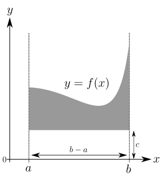
The integral changes by the area of ​​this rectangle of width and height , in formulas ${\displaystyle b-a}$ ${\displaystyle c}$

${\displaystyle \int _{a}^{b}(f(x)+c)\,\mathrm {d} x=\int _{a}^{b}f(x)\,\mathrm {d} x+(b-a)\cdot c.}$

If one looks at a continuous function whose values ​​are negative, one can always find a so that the values in the interval are all positive ( must be greater than the amount of the minimum of in ). With the foregoing consideration one obtains ${\displaystyle c\in \mathbb {R} }$ ${\displaystyle f(x)+c}$ ${\displaystyle c}$ ${\displaystyle f}$ ${\displaystyle [a,b]}$

${\displaystyle \int _{a}^{b}f(x)\,\mathrm {d} x=\int _{a}^{b}(f(x)+c)\,\mathrm {d} x-(b-a)\cdot c,}$

that is, the integral of is the difference between the areas of the white area in the center and the surrounding rectangle. However, this difference is negative, that is, if the above formula is to be correct for any function, areas below the axis must be counted as negative. One speaks therefore of an oriented or directed area. ${\displaystyle f}$ ${\displaystyle x}$

If there are one or more zeros in the interval to be examined, the integral no longer indicates the area, but the sum of the (positive) areas of the partial areas above the -axis and the (negative) areas of the partial areas below the -axis. If you need the area between the -axis and the graph of the function in such an interval , the integral must be divided at the zeros. ${\displaystyle x}$ ${\displaystyle x}$ ${\displaystyle x}$

Cavalieri's principle and the additivity of the integral

→ Main article : Principle of Cavalieri

Axiomatic approach

It is not easy to grasp the concept of area in a mathematically precise way. Various concepts have been developed for this over time. For most applications, however, their details are irrelevant, since, among other things, they agree on the class of continuous functions. In the following, some properties of the integral are listed which were motivated above and which apply to every integral regardless of the exact construction. In addition, they clearly define the integral of continuous functions.

Let it be real numbers and let it be a vector space of functions that includes the continuous functions . Functions in are called "integrable". Then an integral is a map ${\displaystyle a<b}$ ${\displaystyle {\mathcal {F}}}$ ${\displaystyle [a,b]\to \mathbb {R} }$ ${\displaystyle {\mathcal {F}}}$

${\displaystyle {\mathcal {F}}\to \mathbb {R} ,}$

written

${\displaystyle f\mapsto \int _{a}^{b}f(x)\,\mathrm {d} x,}$

with the following characteristics:

• Linearity: For functions and applies ${\displaystyle f,g\in {\mathcal {F}}}$ ${\displaystyle \lambda \in \mathbb {R} }$
  • ${\displaystyle \int _{a}^{b}(f(x)+g(x))\,\mathrm {d} x=\int _{a}^{b}f(x)\,\mathrm {d} x+\int _{a}^{b}g(x)\,\mathrm {d} x}$,
  • ${\displaystyle \int _{a}^{b}\lambda f(x)\,\mathrm {d} x=\lambda \cdot \int _{a}^{b}f(x)\,\mathrm {d} x}$.
• Monotony: Is for everyone , so is ${\displaystyle f(x)\geq 0}$ ${\displaystyle x\in [a,b]}$

  ${\displaystyle \int _{a}^{b}f(x)\,\mathrm {d} x\geq 0.}$

• Integral of the characteristic function of an interval: is an interval and is ${\displaystyle I\subseteq [a,b]}$

${\displaystyle \chi _{I}(x)={\begin{cases}1\ ,&\mathrm {falls} \ x\in I\ ,\\0\ ,&\mathrm {falls} \ x\notin I\ ,\end{cases}}}$

so is

${\displaystyle \int _{a}^{b}\chi _{I}(x)\,\mathrm {d} x}$

equal to the length of the interval . ${\displaystyle I}$

Designations

• The real numbers and are called integration limits. They can be written above and below the integral sign or to the side of the integral sign: ${\displaystyle a}$ ${\displaystyle b}$

${\displaystyle {\textstyle \int \limits _{a}^{b}}f(x)\,{\rm {d}}x}$     or     ${\displaystyle \int \nolimits _{a}^{b}f(x)\,{\rm {d}}x}$

• The function to be integrated is called the integrand . ${\displaystyle f}$
• The variable is called the integration variable . If the integration variable is, one also speaks of integration about . The integration variable is replaceable, instead of ${\displaystyle x}$ ${\displaystyle x}$ ${\displaystyle x}$

${\displaystyle \int _{a}^{b}f(x)\,\mathrm {d} x}$

can be just as good

${\displaystyle \int _{a}^{b}f(t)\,\mathrm {d} t}$ or ${\displaystyle \int _{a}^{b}f(\xi )\,\mathrm {d} \xi }$

write. In the above example, using the letters or leads to undesirable ambiguities, since they already act as identifiers for the integration limits. You should therefore ensure that the character used for the integration variable is not already assigned a different meaning. ${\displaystyle a}$ ${\displaystyle b}$

• The component “ ” is called differential , but in this context mostly has only symbolic meaning. Therefore, no attempt is made here to define it. The integration variable can be read from the differential. ${\displaystyle \mathrm {d} x}$

Origin of the notation

The symbolic notation of integrals goes back to the co-first describer of differential and integral calculus, Gottfried Wilhelm Leibniz . The integral sign ∫ is derived from the letter long s (ſ) for Latin summa . The multiplicative notation indicates how the integral - following the Riemann integral - is made up of strips of height and infinitesimal width . ${\displaystyle f(x)\;\mathrm {d} x}$ ${\displaystyle f(x)}$ ${\displaystyle \mathrm {d} x}$

Alternative spelling in physics

In theoretical physics, for pragmatic reasons, a slightly different notation is often used for integrals (especially for multiple integrals). There is held

${\displaystyle \int _{a}^{b}f(x)\,\mathrm {d} x}$

often

${\displaystyle \int _{a}^{b}\mathrm {d} xf(x)}$

sometimes both spellings are used in different places.

The second example has the disadvantage that the function to be integrated not by and bracketed. In addition, misunderstandings can occur, for example with the Lebesgue integral . However, the alternative notation also has some advantages: ${\displaystyle f(x)}$ ${\displaystyle \textstyle \int _{a}^{b}}$ ${\displaystyle \mathrm {d} x}$

• The expression emphasizes that the integral is a linear operator that acts on everything to the right of it. ${\displaystyle \textstyle \int _{a}^{b}\mathrm {d} x}$
• Integrals often appear in physics in which the function to be integrated is several lines long or it is integrated over several unknowns . Then you already know at the beginning of the integral which variables are integrated and over which limits. Furthermore, the assignment of variables to limits is then easier. ${\displaystyle x_{1},x_{2},\dotsc ,x_{n}}$ ${\displaystyle \textstyle \int _{a}^{b}\mathrm {d} xf(x)}$
• The commutativity of the products in the summands occurring in the Riemann approximation is emphasized. ${\displaystyle \Delta x_{n}\cdot f(x_{n})}$

Example:

${\displaystyle \int _{a_{1}}^{a_{2}}\mathrm {d} t\int _{b_{1}}^{b_{2}}\mathrm {d} x_{1}\int _{c_{1}}^{c_{2}}\mathrm {d} x_{2}\int _{d_{1}}^{d_{2}}\mathrm {d} x_{3}\,f(x_{1},x_{2},x_{3},t)}$

instead of

${\displaystyle \int _{a_{1}}^{a_{2}}\int _{b_{1}}^{b_{2}}\int _{c_{1}}^{c_{2}}\int _{d_{1}}^{d_{2}}f(x_{1},x_{2},x_{3},t)\,\mathrm {d} x_{3}\mathrm {d} x_{2}\mathrm {d} x_{1}\mathrm {d} t}$

Simple consequences of the axioms

• Is for everyone , so is ${\displaystyle f(x)\leq g(x)}$ ${\displaystyle a\leq x\leq b}$

${\displaystyle \int _{a}^{b}f(x)\,\mathrm {d} x\leq \int _{a}^{b}g(x)\,\mathrm {d} x.}$

• If the supremum norm of on is used , then applies ${\displaystyle \|f\|_{\infty }}$ ${\displaystyle f}$ ${\displaystyle [a,b]}$

${\displaystyle \left|\int _{a}^{b}f(x)\,\mathrm {d} x\right|\leq (b-a)\cdot \|f\|_{\infty }.}$

• Is for all with a fixed number , then applies ${\displaystyle |f(x)-g(x)|<\varepsilon }$ ${\displaystyle a\leq x\leq b}$ ${\displaystyle \varepsilon >0}$

${\displaystyle \left|\int _{a}^{b}f(x)\,\mathrm {d} x-\int _{a}^{b}g(x)\,\mathrm {d} x\right|\leq (b-a)\cdot \varepsilon .}$

It follows from this: If a sequence of integrable functions that converges uniformly to an (integrable) function , then is ${\displaystyle (f_{n})_{n\in \mathbb {N} }}$ ${\displaystyle f}$

${\displaystyle \lim _{n\to \infty }\int _{a}^{b}f_{n}(x)\,\mathrm {d} x=\int _{a}^{b}f(x)\,\mathrm {d} x.}$

In other words: the integral is a continuous functional for the supremum norm.

• Integrals of step functions: If a step function , that is, is a disjoint union of intervals of lengths , so that is constant with value , then applies ${\displaystyle f}$ ${\displaystyle [a,b]}$ ${\displaystyle I_{k}}$ ${\displaystyle L_{k}}$ ${\displaystyle f}$ ${\displaystyle I_{k}}$ ${\displaystyle c_{k}}$

${\displaystyle \int _{a}^{b}f(x)\,\mathrm {d} x=\sum _{k=1}^{n}L_{k}\cdot c_{k},}$

thus clearly equal to the sum of the oriented areas of the rectangles between the function graph of and the -axis. ${\displaystyle f}$ ${\displaystyle x}$

Antiderivatives and the main theorem of differential and integral calculus

Integration is an ambiguous reversal of differentiation. To make this more precise, the concept of an antiderivative is needed: If a function is, then a function is called an antiderivative of if the derivative of is equal to : ${\displaystyle f}$ ${\displaystyle F}$ ${\displaystyle f}$ ${\displaystyle F}$ ${\displaystyle f}$

${\displaystyle F'=f}$

This reversal is ambiguous because different functions (e.g. polynomial functions that differ only in the Y-axis intercept) can have one and the same derivative, which means that a function has not just one but an infinite number of antiderivatives.

The main theorem of differential and integral calculus establishes the relationship between antiderivatives and integrals. It says: If is a continuous function on an interval and is an antiderivative of , then we have ${\displaystyle f}$ ${\displaystyle [a,b]}$ ${\displaystyle F}$ ${\displaystyle f}$

${\displaystyle \int _{a}^{b}f(x)\,\mathrm {d} x=F(b)-F(a).}$

The right side is often abbreviated as

${\displaystyle [F(x)]_{a}^{b}=[F(x)]_{x=a}^{x=b}=F(x){\Big |}_{a}^{b}=F(x){\Big |}_{x=a}^{x=b}}$ or similar

written.

This relationship is the main method for the explicit evaluation of integrals. The difficulty usually lies in finding an antiderivative.

The mere existence is theoretically secured: the integral function

${\displaystyle x\mapsto \int _{a}^{x}f(t)\,\mathrm {d} t}$

is for each an antiderivative of . ${\displaystyle a}$ ${\displaystyle f}$

Properties of antiderivatives

You can add a constant to an antiderivative and get an antiderivative again: If an antiderivative is to a function and is a constant, then is ${\displaystyle F}$ ${\displaystyle f}$ ${\displaystyle c\in \mathbb {R} }$

${\displaystyle (F+c)'=F\!\,'+0=F'=f.}$

Two antiderivatives of the same function defined on an interval differ by a constant: If and antiderivatives of the same function , then is ${\displaystyle F}$ ${\displaystyle G}$ ${\displaystyle f}$

${\displaystyle (F-G)\!\,'=F'-G'=f-f=0,}$

so the difference is a constant. If the domain of is not an interval, the difference between two antiderivatives is only locally constant . ${\displaystyle F-G}$ ${\displaystyle f}$

Indefinite integral

An antiderivative is also known as the indefinite integral of - but sometimes it also means the set of all antiderivatives. If it is an antiderivative, it is often written imprecisely ${\displaystyle f(x)}$ ${\displaystyle F(x)}$

${\displaystyle \int f(x)\,\mathrm {d} x=F(x)+C,}$

to indicate that every antiderivative of has the form with a constant . The constant is called the constant of integration. ${\displaystyle f}$ ${\displaystyle F(x)+C}$ ${\displaystyle C}$ ${\displaystyle C}$

Note that the notation

${\displaystyle \int f(x)\,\mathrm {d} x}$

however, it is also often used in formulas to indicate that equations hold for arbitrary, consistently chosen limits; for example is with

${\displaystyle \int cf(x)\,\mathrm {d} x=c\int f(x)\,\mathrm {d} x}$

meant that

${\displaystyle \int _{a}^{b}cf(x)\,\mathrm {d} x=c\int _{a}^{b}f(x)\,\mathrm {d} x}$

holds for any . ${\displaystyle a,b}$

Determination of antiderivatives

See also the article: Table of derivative and antiderivatives or indefinite integrals in the mathematics formula collection .

In contrast to the derivative function, the explicit calculation of an antiderivative is very difficult or not possible for many functions. This is why integrals are often looked up in tables (e.g. an integral table ). For the manual calculation of an antiderivative, the skillful use of the following standard techniques is often helpful.

Partial integration

→ Main article : Partial integration

Partial integration is the reverse of the product rule of differential calculus. It is:

${\displaystyle \int _{a}^{b}f'(x)\cdot g(x)\,\mathrm {d} x=[f(x)\cdot g(x)]_{a}^{b}-\int _{a}^{b}f(x)\cdot g'(x)\,\mathrm {d} x}$

This rule is useful when the function is easier to integrate than the function . Here, however, the products and not the factors themselves are to be assessed. ${\displaystyle f(x)\cdot g'(x)}$ ${\displaystyle f'(x)\cdot g(x)}$

Example:

${\displaystyle \int _{a}^{b}x\ln(x)\,\mathrm {d} x}$

If you set

${\displaystyle f'(x)=x\,}$ and ${\displaystyle g(x)=\ln(x)\,}$

so is

${\displaystyle f(x)={\frac {x^{2}}{2}}}$ and ${\displaystyle g'(x)={\frac {1}{x}}}$

and one receives

${\displaystyle {\begin{aligned}\int _{a}^{b}x\ln(x)\,\mathrm {d} x&={\frac {b^{2}}{2}}\ln(b)-{\frac {a^{2}}{2}}\ln(a)-\int _{a}^{b}{\frac {x^{2}}{2}}\cdot {\frac {1}{x}}\,\mathrm {d} x\\&={\frac {b^{2}}{2}}\left(\ln(b)-{\frac {1}{2}}\right)-{\frac {a^{2}}{2}}\left(\ln(a)-{\frac {1}{2}}\right).\end{aligned}}}$

Integration through substitution

→ Main article : Integration through substitution

The substitution rule is an important tool for calculating some difficult integrals, as it allows certain changes to the function to be integrated while changing the integration limits. It is the counterpart to the chain rule in differential calculus.

Let with and be an antiderivative of , then is an antiderivative of , because it holds ${\displaystyle \varphi (x)=f(g(x))\cdot g'(x)}$ ${\displaystyle g'\neq 0}$ ${\displaystyle F}$ ${\displaystyle f}$ ${\displaystyle \Phi (x)=F(g(x))}$ ${\displaystyle \varphi }$

${\displaystyle {\frac {\varphi (x)}{g'(x)}}=f(g(x))}$

and with the substitution

${\displaystyle z=g(x),\quad \mathrm {d} z=g'(x)\mathrm {d} x}$

finally

${\displaystyle {\begin{aligned}\int _{a}^{b}f(g(x))g'(x)\mathrm {d} x&=\int _{g(a)}^{g(b)}f(z)\mathrm {d} z\\&=F(g(b))-F(g(a))\\&=\Phi (b)-\Phi (a).\end{aligned}}}$

Reshaping by partial fraction decomposition

In the case of fractional-rational functions, a polynomial division or a partial fraction decomposition often leads to a transformation of the function, which allows one of the integration rules to be applied.

Special procedures

It is often possible to determine the antiderivative using the special form of the integrand.

Another possibility is to start with a known integral and transform it using integration techniques until the desired integral is obtained. Example:

To determine, we partially integrate the following similar integral: ${\displaystyle \textstyle \int {\frac {\mathrm {d} x}{(1+x^{2})^{2}}}}$

${\displaystyle {\begin{aligned}\arctan x&=\int 1\cdot {\frac {1}{1+x^{2}}}\,\mathrm {d} x\\&=x\cdot {\frac {1}{1+x^{2}}}+\int x\cdot {\frac {2x}{(1+x^{2})^{2}}}\,\mathrm {d} x\\&={\frac {x}{1+x^{2}}}+\int \left({\frac {2x^{2}}{(1+x^{2})^{2}}}+{\frac {2}{(1+x^{2})^{2}}}\right)\,\mathrm {d} x-\int {\frac {2}{(1+x^{2})^{2}}}\,\mathrm {d} x\\&={\frac {x}{1+x^{2}}}+2\int {\frac {1+x^{2}}{(1+x^{2})^{2}}}\,\mathrm {d} x-2\int {\frac {1}{(1+x^{2})^{2}}}\,\mathrm {d} x\\&={\frac {x}{1+x^{2}}}+2\arctan x-2\int {\frac {\mathrm {d} x}{(1+x^{2})^{2}}}\end{aligned}}}$

By moving follows

${\displaystyle \int {\frac {\mathrm {d} x}{(1+x^{2})^{2}}}={\frac {1}{2}}\left({\frac {x}{1+x^{2}}}+\arctan x\right).}$

Applications

Mean values ​​of continuous functions

To calculate the mean value of a given continuous function on an interval, one uses the formula ${\displaystyle m}$ ${\displaystyle f}$ ${\displaystyle [a,b]}$

${\displaystyle m={\frac {1}{b-a}}\int _{a}^{b}f(x)\mathrm {d} x.}$

Since this definition for staircase functions corresponds to the usual concept of mean value, this generalization makes sense.

The mean value theorem of integral calculus says that this mean value is actually assumed by a continuous function in the interval . ${\displaystyle [a,b]}$

Example of the term integral in physics

A physical phenomenon that can be used to explain the term integral is the free fall of a body in the earth's gravitational field . The acceleration of free fall in Central Europe is approx. 9.81 m / s². The speed of a body at the time can therefore be expressed by the formula ${\displaystyle g}$ ${\displaystyle v}$ ${\displaystyle t}$

${\displaystyle v=g\cdot t}$

express.

But now the distance that the falling body covers within a certain time should be calculated . The problem here is that the body's speed increases over time. To solve the problem, it is assumed that for a short period of time the speed , which results from time , remains constant. ${\displaystyle l}$ ${\displaystyle T}$ ${\displaystyle v}$ ${\displaystyle \Delta t}$ ${\displaystyle v}$ ${\displaystyle g\cdot t}$

The increase in distance within the short period is therefore ${\displaystyle \Delta t}$

${\displaystyle \Delta l=g\cdot t\,\cdot \Delta t}$.

The entire distance can therefore be described as

${\displaystyle l=\sum \left(g\cdot t\,\cdot \Delta t\right)}$

express. If one now lets the time difference tend towards zero, one obtains ${\displaystyle \Delta t}$

${\displaystyle l=\lim _{\Delta t\to 0}\left(\sum \left(g\cdot t\,\cdot \Delta t\right)\right)=\int _{0}^{T}\left(g\cdot t\;\mathrm {d} t\,\right).}$

The integral can be given analytically with

${\displaystyle l=\,{\frac {g}{2}}\cdot T^{2}.}$

The general solution leads to the equation of motion of the body falling in the constant gravitational field:

${\displaystyle l={\frac {g}{2}}\cdot t^{2}}$

From this equation of motion, by differentiating according to time, the equation for the speed can be:

${\displaystyle v=g\cdot t}$

and derive by differentiating again for the acceleration:

${\displaystyle a=g}$

Other simple examples are:

• The energy is the integral of the power over time.
• The electrical charge of a capacitor is the integral of the current flowing through it over time.
• The integral of the product of the spectral irradiance ( E _e (ν) in W / m ² Hz ) with the spectral light sensitivity curve of the eye provides the illuminance ( E in lux = lumen / m ² ).
• The integral of the flow velocity (longitudinal component) over the cross-section of a pipe provides the entire volume flow through the pipe ( see below for further multi-dimensional integrals ).

Constructions

Cauchy integral

Augustin-Louis Cauchy

A control function is a function that can be approximated evenly using step functions . Due to the aforementioned compatibility of the integral with uniform limits, one can define the integral for a control function that is the uniform limit of a sequence of step functions as ${\displaystyle f}$ ${\displaystyle t_{n}}$

${\displaystyle \int _{a}^{b}f(x)\,\mathrm {d} x=\lim _{n\to \infty }\int _{a}^{b}t_{n}(x)\,\mathrm {d} x,}$

where the integral for step functions is defined by the formula given above.

The class of control functions includes all continuous functions and all monotonic functions , as well as all functions for which can be subdivided into a finite number of intervals , so that the restriction from to a continuous or monotonic function is on the closed interval , i.e. H. all piecewise continuous functions. It also includes functions of limited variation , since such a function can be represented as the difference between two monotonically increasing functions. This integral construction is completely sufficient for many practical purposes. ${\displaystyle f}$ ${\displaystyle [a,b]}$ ${\displaystyle I_{k}}$ ${\displaystyle f}$ ${\displaystyle I_{k}}$ ${\displaystyle {\bar {I}}_{k}}$

There are also continuous functions with infinite variation such as B. the function defined by and for on the interval (see variation ). ${\displaystyle 0\mapsto 0}$ ${\displaystyle t\mapsto t\cos {\tfrac {\pi /2}{t}}}$ ${\displaystyle 0<t\leq 1}$ ${\displaystyle [0,1]}$

Riemann integral

→ Main article : Riemann's integral

Bernhard Riemann

One approach to calculating the integral according to Riemann is to approximate the function to be integrated by a step function ; however, not by uniform approximation of the function itself, but by approximation of the area by means of rectangular sums.

The area is approximated by the sum of the areas of the individual rectangles under the individual "steps". For each breakdown of the integration interval, you can choose any function value within each sub-interval as the level of the level.

These are after the German mathematician Bernhard Riemann called Riemann sums. If one chooses the supremum of the function as the height of the rectangle in each sub-interval of the decomposition , then the upper sum results, with the infimum the lower sum.

The Riemann integral can be defined with the help of upper and lower sums, see Riemann integral. If the upper and lower sums converge to the same limit value , this limit value is the integral in the Riemann sense. Integrable in this sense are z. B. all functions for which the Cauchy integral exists.

The Riemann integral exists e.g. B. not for the indicator function of the rational numbers in the interval , i. H. for the Dirichlet function . Therefore, extended integral terms were introduced by Henri Léon Lebesgue ( Lebesgue integral ), Thomas Jean Stieltjes ( Stieltjesintegral ) and Alfréd Haar , which reproduce the Riemann integral for continuous integrands. ${\displaystyle [0,1]}$

Stieltjes integral

→ Main article : Stieltjes integral

The Stieltjes integral is based on monotonic functions , or those with finite variation , that is, differences between two monotonic functions, and Riemann-Stieltjes sums are defined for continuous functions as ${\displaystyle g(x)}$ ${\displaystyle f}$

${\displaystyle \sum _{i=0}^{n-1}\,f(x_{i})\,\{g(x_{i+1})-g(x_{i})\}.}$

The so-called Riemann-Stieltjes integral is then obtained by forming a limit in the usual way . ${\displaystyle \textstyle \int _{I}\,f\,\mathrm {d} g}$

Such integrals are also defined if the function is not differentiable (otherwise applies ). A well-known counterexample is the so-called Heaviside function , the value of which is zero for negative numbers, one for positive and z. B. for the point . One writes for and thus receives the “generalized function” , the so-called Dirac measure , as a measure only defined for the point . ${\displaystyle g}$ ${\displaystyle \mathrm {d} g\equiv g'(x)\,\mathrm {d} x}$ ${\displaystyle \Theta (x)}$ ${\displaystyle x}$ ${\displaystyle =1/2}$ ${\displaystyle x=0}$ ${\displaystyle g(x)=\Theta (x),}$ ${\displaystyle \mathrm {d} g=\delta (x)\mathrm {d} x}$ ${\displaystyle \delta (x)}$ ${\displaystyle x=0}$

Lebesgue integral

→ Main article : Lebesgue integral

Henri Lebesgue

The Lebesgue integral provides a more modern and - in many ways - better integral term than that of the Riemann integral. For example, it allows integration using general dimensional spaces . This means that quantities can be assigned a measure that does not necessarily have to match their geometric length or volume, such as probability measures in probability theory . The measure that corresponds to the intuitive concept of length or volume is the Lebesgue measure . As a rule, the integral over this dimension is referred to as the Lebesgue integral . One can prove that for every function that is Riemann integrable over a compact interval, the corresponding Lebesgue integral also exists and the values ​​of both integrals agree. Conversely, however, not all Lebesgue-integrable functions are also Riemann-integrable. The best-known example of this is the Dirichlet function , i.e. the function that has the value one for rational numbers but the value zero for irrational numbers. In addition to the larger class of integrable functions, the Lebesgue integral is distinguished from the Riemann integral primarily by the better convergence theorems ( theorem of monotonic convergence , theorem of majorized convergence ) and the better properties of the function spaces normalized by the Lebesgue integral (approximately completeness ).

In modern mathematics, integral or integration theory is often understood as Lebesgue's integral term.

Improper integral

→ Main article : improper integral

The Riemann integral is (in one-dimensional space) only defined for compact , i.e. restricted and closed , intervals. The improper integral offers a generalization to unlimited domains of definition or functions with singularities . In the Lebesgue theory, improper integrals can also be considered, but this is not so productive, since the Lebesgue integral can already integrate many functions with singularities or an unlimited domain.

Method for calculating definite and improper integrals

Numerical methods

It is often difficult or not possible to specify an antiderivative explicitly. However, in many cases it is sufficient to calculate the specific integral approximately. One then speaks of numerical quadrature or numerical integration . Many methods for numerical quadrature are based on an approximation of the function using functions that can be easily integrated, for example using polynomials. The trapezoidal rule or the Simpson's formula (the special case of which is known as Kepler's barrel rule ) are examples of this, here an interpolation polynomial is placed by the function and then integrated.

Long before the spread of computers, methods for automatic step size control were developed for numerical integration . Today, computer algebra offers the possibility of numerically solving complex integrals in ever shorter times or with ever more precise solutions, although there are still difficulties with improper integrals for the calculation of which special methods such as Gauss-Kronrod often have to be used. An example of such a hard integral is:

${\displaystyle \int _{0}^{\infty }{\frac {\ln(1+x)}{\ln ^{2}x+\pi ^{2}}}\cdot {\frac {\mathrm {d} x}{x^{2}}}=\gamma }$

Classic methods are e.g. B. Euler's empirical formula , in which the definite integral is approximated by a generally asymptotic series . Other methods are based on the theory of difference calculus , an important example here is the Gregory integration formula.

Exact procedures

Leonhard Euler

David Bierens de Haan

There are a number of methods with which definite and improper integrals can be calculated exactly in symbolic form.

If continuous and an antiderivative is known, the definite integral can be ${\displaystyle f}$ ${\displaystyle f}$ ${\displaystyle F}$

${\displaystyle \int _{a}^{b}f(x)\,\mathrm {d} x=F(b)-F(a)}$

calculate by the main clause. The problem is that the operation of the indefinite integration leads to an extension of given functional classes. For example, the integration within the class of the rational functions is not complete and leads to the functions and . The class of so-called elementary functions is not closed either. Thus Joseph Liouville proved that the function has no elementary antiderivative. Leonhard Euler was one of the first to develop methods for the exact calculation of certain and improper integrals without determining an antiderivative. Over time, numerous more general and specific methods of specific integration have emerged: ${\displaystyle \ln }$ ${\displaystyle \arctan }$ ${\displaystyle e^{-x^{2}}}$

• Using the residual theorem
• Representation of the integral depending on a parameter using special functions
• Differentiation or integration of the integral according to a parameter and interchanging the boundary processes
• Use of a series expansion of the integrand with integration by term
• reduce the integral to itself or to another through partial integration and substitution

By the end of the 20th century, numerous (sometimes multi-volume) integral tables with certain integrals had been created. A few examples to illustrate the problem:

${\displaystyle \int _{0}^{1}{\frac {\ln(1+x)}{x^{2}+1}}\,\mathrm {d} x={\frac {\pi }{8}}\ln 2}$

${\displaystyle \int _{0}^{\pi }\ln \sin x\,\mathrm {d} x=-\pi \ln 2}$

Special integrals

There are a number of definite and improper integrals that have a certain meaning for mathematics and therefore have their own name:

• Euler's integrals of the first and second kind
• Gaussian error integral

${\displaystyle \int _{-\infty }^{\infty }e^{-t^{2}}\,\mathrm {d} t={\sqrt {\pi }}}$

• Fresnel integrals

${\displaystyle \int _{0}^{\infty }\cos t^{2}\,\mathrm {d} t=\int _{0}^{\infty }\sin t^{2}\,\mathrm {d} t={\tfrac {1}{4}}{\sqrt {2\pi }}}$

• Raabe's integral

${\displaystyle \int \limits _{a}^{a+1}\log \Gamma (t)\,\mathrm {d} t={\tfrac {1}{2}}\log 2\pi +a\log a-a,\quad a\geq 0,}$   and especially for and  : ${\displaystyle a=0}$ ${\displaystyle a=e}$ ${\displaystyle \int _{0}^{1}\log \Gamma (t)\,\mathrm {d} t={\tfrac {1}{2}}\log 2\pi }$

• Frullan integrals

${\displaystyle \int _{0}^{\infty }{\frac {f(ax)-f(bx)}{x}}\,\mathrm {d} x}$

Multi-dimensional integration

Path integrals

→ Main article : Curve integral

Real path integrals and length of a curve

If there is a path , i.e. a continuous mapping, and a scalar function, then the path integral of along is defined as ${\displaystyle \gamma \colon [a,b]\to \mathbb {R} ^{n}}$ ${\displaystyle f\colon \mathbb {R} ^{n}\to \mathbb {R} }$ ${\displaystyle f}$ ${\displaystyle \gamma }$

${\displaystyle \int _{\gamma }f(x)\,\mathrm {d} x=\int _{a}^{b}f(\gamma (t))\,\|{\dot {\gamma }}(t)\|\,\mathrm {d} t.}$

If , we get the length of the curve (physically speaking) from the above formula as the integral of the speed over time: ${\displaystyle f\equiv 1}$ ${\displaystyle \gamma \colon [a,b]\to \mathbb {R} ^{2}}$

${\displaystyle L(\gamma )=\int _{a}^{b}\|{\dot {\gamma }}(t)\|\,\mathrm {d} t=\int _{a}^{b}{\sqrt {{\dot {x}}(t)^{2}+{\dot {y}}(t)^{2}}}\,\mathrm {d} t}$

Real path integrals for vector functions

Path integrals of the following form are often used in physics: is a vector function , and it becomes the integral ${\displaystyle {\vec {f}}}$ ${\displaystyle \mathbb {R} ^{n}\to \mathbb {R} ^{n}}$

${\displaystyle \int _{\gamma }{\vec {f}}(x)\cdot \mathrm {d} x=\int _{a}^{b}\langle {\vec {f}}(\gamma (t)),{\dot {\gamma }}(t)\rangle \,\mathrm {d} t}$

considered, with the expression in the angled brackets being a scalar product .

Complex path integrals

In function theory , i.e. the expansion of analysis to include functions of a complex variable, it is no longer sufficient to specify lower and upper integration limits. Unlike two points on the number line, two points on the complex plane can be connected to one another in many ways. Therefore the definite integral in function theory is basically a path integral . The residual theorem applies to closed paths , an important result of Cauchy: The integral of a meromorphic function along a closed path depends solely on the number of enclosed singularities. It is zero if there are no singularities in the integration area.

Surface integrals

→ Main article : Surface integral

Example: Calculation of room contents

As an example, the volume between the graph of the function is calculated with over the unit square . To do this, one divides the integral over into two integrals, one for the - and one for the - coordinate: ${\displaystyle f\colon \mathbb {R} ^{2}\to \mathbb {R} }$ ${\displaystyle f(x,y):=x^{2}+y}$ ${\displaystyle I:=[0,1]\times [0,1]}$ ${\displaystyle I}$ ${\displaystyle x}$ ${\displaystyle y}$

${\displaystyle {\begin{aligned}\int _{[0,1]\times [0,1]}f(x,y)\,\mathrm {d} (x,y)&=\int _{0}^{1}\int _{0}^{1}f(x,y)\,\mathrm {d} x\,\mathrm {d} y=\int _{0}^{1}\int _{0}^{1}(x^{2}+y)\,\mathrm {d} x\,\mathrm {d} y\\&=\int _{0}^{1}\left[{\tfrac {1}{3}}x^{3}+yx\right]_{x=0}^{1}\,\mathrm {d} y=\int _{0}^{1}\left({\tfrac {1}{3}}+y\right)\mathrm {d} y=\left[{\tfrac {1}{3}}y+{\tfrac {1}{2}}y^{2}\right]_{y=0}^{1}={\tfrac {5}{6}}\end{aligned}}}$

For the surface integral gives the area of ​​the integration surface. ${\displaystyle f\equiv 1}$

Volume integrals

→ Main article : Volume integral

For the volume integral calculates the volume of the integration area. ${\displaystyle f\equiv 1}$

Integration across multi-dimensional and higher-dimensional areas

The concept of integral can be generalized to the case that the carrier set on which the integrand operates is not the number line , but the -dimensional Euclidean space . ${\displaystyle f}$ ${\displaystyle \mathbb {R} }$ ${\displaystyle n}$ ${\displaystyle \mathbb {R} ^{n}}$

Fubini's theorem and transformation theorem

For multi-dimensional integrals, i.e. also area and volume integrals, Fubini's theorem is used, which allows the integrals to be split up in any order over the individual coordinates and processed one after the other:

${\displaystyle {\begin{aligned}\int _{V}f\left({\vec {r}}\right)\mathrm {d} ^{3}r&=\iiint f(x,y,z)\mathrm {d} z\,\mathrm {d} y\,\mathrm {d} x\\&=\int \left(\int \left(\int f(x,y,z)\mathrm {d} z\right)\mathrm {d} y\right)\mathrm {d} x\end{aligned}}}$

The integration limits of the one-dimensional integrals in , and must be determined from the limitation of the volume . Analogous to the improper integrals in the one-dimensional (see above) one can also consider integrals over the entire, unrestricted -dimensional space. ${\displaystyle x}$ ${\displaystyle y}$ ${\displaystyle z}$ ${\displaystyle V}$ ${\displaystyle n}$

The generalization of the rule of substitution in the multidimensional is the transformation theorem . Be open and an injective , continuously differentiable mapping whose functional determinant applies to all . Then ${\displaystyle \Omega \subset \mathbb {R} ^{d}}$ ${\displaystyle \Phi \colon \Omega \to \mathbb {R} ^{d}}$ ${\displaystyle \det(D\Phi (x))\neq 0}$ ${\displaystyle x\in \Omega }$

${\displaystyle \int _{\Phi (\Omega )}f(y)\,\mathrm {d} y=\int _{\Omega }f(\Phi (x))\left|\det(D\Phi (x))\right|\mathrm {d} x.}$

Integrals over manifolds

Integration over the surface of an area is particularly interesting in many physical applications. Such surfaces are usually described by manifolds . These are described by so-called maps.

Integration over a map area

Let be a -dimensional submanifold of and a map area in , i.e. an open subset in , for which there is a map that maps it diffeomorphically onto an open subset of . Furthermore, let a parameterization of , i.e. a continuously differentiable mapping, the derivation of which has full rank, which maps homeomorphically to . Then the integral of a function in the map area is defined as follows: ${\displaystyle M}$ ${\displaystyle d}$ ${\displaystyle \mathbb {R} ^{n}}$ ${\displaystyle U}$ ${\displaystyle M}$ ${\displaystyle M}$ ${\displaystyle \mathbb {R} ^{d}}$ ${\displaystyle \gamma \colon \Omega \to U}$ ${\displaystyle U}$ ${\displaystyle \Omega }$ ${\displaystyle \gamma (\Omega )}$ ${\displaystyle U}$

${\displaystyle \int _{U}f\mathrm {d} s:=\int _{\Omega }f(\gamma (u)){\sqrt {g^{\gamma }(u)}}\mathrm {d} u,}$

where is the Gram's determinant . The right integral can be calculated using the methods of multidimensional integration described above. The equality essentially follows from the transformation theorem. ${\displaystyle g^{\gamma }(u)=\det((\gamma '(u))^{\mathsf {T}}\cdot \gamma '(u))}$

Integration over a submanifold

If there is a breakdown of 1 that is compatible with the maps of the submanifold, it can simply be integrated and added up separately over the map areas.

The Gaussian integral theorem and the Stokes theorem

For special functions, the integrals can be calculated more easily using submanifolds. Two statements are particularly important in physics:

On the one hand, the Gaussian integral theorem , according to which the volume integral over the divergence of a vector field is equal to the surface integral over the vector field (the flow of the field through the surface): Be compact with a smooth edge in sections . Let the edge be oriented by an outer normal unit field . Furthermore, let be a continuously differentiable vector field on an open neighborhood of . Then applies ${\displaystyle V\subset \mathbb {R} ^{n}}$ ${\displaystyle \partial V}$ ${\displaystyle {\vec {n}}}$ ${\displaystyle {\vec {F}}}$ ${\displaystyle V}$

${\displaystyle \int _{V}\operatorname {div} {\vec {F}}\,\mathrm {d} ^{(n)}V=\oint _{\partial V}{\vec {F}}\cdot \mathrm {d} ^{(n-1)}{\vec {S}}}$

with the abbreviation . ${\displaystyle \mathrm {d} ^{(n-1)}{\vec {S}}={\vec {n}}\,\mathrm {d} ^{(n-1)}S}$

With this theorem, the divergence is interpreted as the so-called source density of the vector field. The dimension of the respective integration manifold is additionally emphasized by the indices or the operator. ${\displaystyle (n)}$ ${\displaystyle (n-1)}$ ${\displaystyle \mathrm {d} }$

If multiple integrals are used explicitly (without indexing), for : ${\displaystyle n=3}$

${\displaystyle \iiint _{V}\operatorname {div} \,{\vec {F}}({\vec {x}})\,\mathrm {d} V=\iint _{\partial V}{\vec {F}}\cdot \mathrm {d} {\vec {S}}}$

So: The integral of the divergence over the entire volume is equal to the integral of the flow from the surface.

Second, Stokes ' theorem , which is a statement of differential geometry and, in the special case of three-dimensional space, can be written directly with multiple integrals.

If there is a two-dimensional submanifold of three-dimensional Euclidean space , then applies ${\displaystyle M}$ ${\displaystyle \mathbb {R} ^{3}}$

${\displaystyle \iint _{M}\operatorname {rot} {\vec {F}}\cdot \mathrm {d} {\vec {S}}=\int _{\partial M}{\vec {F}}\cdot \mathrm {d} {\vec {r}},}$

where denotes the rotation of the vector field . ${\displaystyle \operatorname {rot} {\vec {F}}}$ ${\displaystyle {\vec {F}}}$

This sentence interprets the rotation of a vector field as the so-called vortex density of the vector field; where the three-component vector and the edge of a closed curve is im . ${\displaystyle \mathrm {d} {\vec {r}}}$ ${\displaystyle (\mathrm {d} x,\mathrm {d} y,\mathrm {d} z)}$ ${\displaystyle \partial M}$ ${\displaystyle M}$ ${\displaystyle \mathbb {R} ^{3}}$

Integration of vector-valued functions

The integration of functions that are not real or complex-valued but take on values ​​in a more general vector space is also possible in a wide variety of ways.

The direct generalization of the Lebesgue integral to Banach space-valued functions is the Bochner integral (after Salomon Bochner ). Many results of the one-dimensional theory are literally transferred to Banach spaces.

Transferring the definition of the Riemann integral to vector-valued functions using Riemann sums is also not difficult. A crucial difference here, however, is that not every Riemann-integrable function can then be Bochner-integrable. ${\displaystyle f\colon [a,b]\to V}$

A common generalization of the Bochner and Riemann integrals that overcomes this deficiency is the McShane integral , which can be most easily defined using generalized Riemann sums.

The Birkhoff integral is also a common generalization of the Bochner and Riemann integral. In contrast to the McShane integral, the definition of the Birkhoff integral does not require a topological structure in the definition area of ​​the functions. However, if the requirements for McShane integration are met, every Birkhoff-integrable function can also be McShane-integrable.

In addition, the Pettis integral is worth mentioning as the next step in generalization. It uses a functional analytical definition in which the integrability is traced back to the one-dimensional case: Let it be a measure space . A function is called Pettis-integrable if the function Lebesgue-integrable for every continuous functional and a vector exists for every measurable set , so that ${\displaystyle (\Omega ,{\mathcal {A}},\mu )}$ ${\displaystyle f\colon \Omega \to V}$ ${\displaystyle \lambda \in V'}$ ${\displaystyle \lambda \circ f\colon \Omega \to \mathbb {R} }$ ${\displaystyle A\in {\mathcal {A}}}$ ${\displaystyle x_{A}\in V}$

${\displaystyle \forall \lambda \in V'\colon \ \lambda (x_{A})=\int _{A}{\lambda \circ f}\,\mathrm {d} \mu }$

applies. The vector is then appropriately labeled. ${\displaystyle x_{A}}$ ${\displaystyle \textstyle \int _{A}f\,\mathrm {d} \mu }$

For functions that take values ​​in a separable Banach space , the Pettis integral agrees with the McShane and Bochner integrals. The most important special case of all these definitions is the case of functions in the , which are simply integrated component by component in all of these definitions. ${\displaystyle f\colon [a,b]\to V}$ ${\displaystyle V}$ ${\displaystyle \mathbb {R} ^{n}}$

Generalizations

The term integral has been expanded in many ways, some variants are:

• Riemann integral
• Daniell integral
• Stieltjes integral
• Itō integral and Stratonowitsch integral , see also Diskretes_stochastisches_Integral
• Gauge integral or Henstock-Kurzweil integral , especially:
  • McShane integral
  • Pepper integral
• Measure integral
  • Lebesgue integral
  • Bochner integral
  • Birkhoff integral
  • Pettis integral
  • Hair integral
• Volkenborn integral

Measure theory

→ Main article : Measure theory

Hairy measure

→ Main article : Haarsches Maß

The Haar measure, after Alfréd Haar , represents a generalization of the Lebesgue measure for locally compact topological groups and thus also induces an integral as a generalization of the Lebesgue integral.

Integration on manifolds

See: Integration of differential forms

Finally, integration can also be used to measure surfaces of given bodies. This leads into the field of differential geometry .

See also

• Algebraic integration
• Stochastic integration
• Table of derivative and antiderivatives
• Volkenborn integral

literature

• School books:
  • Integral calculus is a central subject in the upper secondary level and is therefore dealt with in all mathematics textbooks.
• Textbooks for students of mathematics and related subjects (physics, computer science):
  • Herbert Amann, Joachim Escher : Analysis I, II, III. Birkhäuser-Verlag Basel Boston Berlin, ISBN 3-7643-7755-0 , ISBN 3-7643-7105-6 , ISBN 3-7643-6613-3 .
  • Richard Courant : Lectures on differential and integral calculus 1, 2nd Springer, 1st edition 1928, 4th edition 1971.
  • Gregor Michailowitsch Fichtenholz : Differential and Integral Calculus I – III. Harri Deutsch publishing house, Frankfurt am Main, 1990–2004. ISBN 978-3-8171-1418-4 (complete set).
  • Otto Forster : Analysis 1. Differential and integral calculus of a variable. 7th edition. Vieweg-Verlag, 2004. ISBN 3-528-67224-2 .
  • Otto Forster: Analysis. Volume 3: Measure and integration theory, integral theorems in R ⁿ and applications , 8th improved edition. Springer Spectrum, Wiesbaden, 2017, ISBN 978-3-658-16745-5 .
  • Konrad Königsberger : Analysis. 2 volumes, Springer, Berlin 2004.
  • Vladimir Ivanovich Smirnov : Course in higher mathematics (part 1–5). Harri Deutsch publishing house, Frankfurt am Main, 1995–2004. ISBN 978-3-8171-1419-1 (complete set).
  • Steffen Timmann: Repetitorium der Analysis 1, 2nd 1st edition. Binomi Verlag, 1993.
• Textbooks for students with a minor / basic subject in mathematics (for example engineering or economics students):
  • Rainer Ansorge and Hans Joachim Oberle: Mathematics for Engineers. Volume 1. 3rd edition. Wiley-VCH, 2000.
  • Lothar Papula : Mathematics for natural scientists and engineers. Volume 1. 13th edition. Vieweg + Teubner Verlag. ISBN 978-3-8348-1749-5 .
• Historical:
  • Adolph Mayer: Contributions to the theory of the maxima and minima of simple integrals. Teubner, Leipzig 1866 ( digitized version ).
  • Bernhard Riemann: About the representability of a function by a trigonometric series. Göttingen 1867 ( full text ), with the first definition of the Riemann integral (page 12 ff.).

Web links

Wikibooks: Introduction to Integral calculus  - learning and teaching materials

Wiktionary: Integral calculus  - explanations of meanings, word origins, synonyms, translations

• Online calculator for calculating integrals (antiderivatives) with calculation method and explanations (German)
• mathe-online.at - Resources on the topic of integration (secondary level 2 / FHS / Uni)
• Clear explanations
• The Integrator - English page for calculating integrals
• Integral calculator - German site for the calculation of definite and indefinite integrals (antiderivatives)
• Part 1 of a three-part series on multiple integrals (detailed + extensive)
• 50 examples of primitive functions of functions
• Video: integral, antiderivative . Jörn Loviscach 2010, made available by the Technical Information Library (TIB), doi : 10.5446 / 9752 .
• Video: derivative, integral, chance . Jörn Loviscach 2010, made available by the Technical Information Library (TIB), doi : 10.5446 / 9736 .
• Video: definite integral 1 . Jörn Loviscach 2010, made available by the Technical Information Library (TIB), doi : 10.5446 / 9755 .
• Video: definite integral 2 . Jörn Loviscach 2010, made available by the Technical Information Library (TIB), doi : 10.5446 / 9756 .

Individual evidence

1. ↑ D. Fremlin: The McShane and Birkhoff integrals of vector-valued functions. ( Memento from April 28, 2015 in the Internet Archive )