
Fluorescence microscopy

Fluorescence microscopy is a special form of light microscopy . It is based on the physical effect of fluorescence . When fluorescent substances are excited with light of certain wavelengths , they emit light of other, longer wavelengths ( Stokes shift ).
With fluorescence microscopy, the generated, enlarged image of the examined object is generated only by radiated (emitted) light. Color filters prevent excitation light from reaching the image. Fluorescence microscopic images are informative if the entire microscopic specimen does not fluoresce evenly, but only some structures light up. These structures generate light signals against a dark background.
Every fluorescent molecule in the preparation can be viewed as a new light source. If the intensity of the fluorescence emitted by these molecules is above the detection limit, structures that are much smaller than the resolution limit of the microscope can also be detected with fluorescence microscopy. The resolution limit is not overcome with classical fluorescence microscopy, since detection is possible at a small distance, but no statement as to whether the signal is caused by one or more structures. In this respect it is similar to dark field microscopy .
In addition to the classic, there are numerous further developed special forms of fluorescence microscopy. These include, for example, confocal laser scanning microscopy and multi-photon fluorescence microscopy . From the 1990s onwards, various methods were developed that actually enable a significantly improved resolution. These so-called ultra-resolution or super-resolution methods are also of the fluorescence microscopic type.
Basics
fluorescence


A fluorescent molecule has an electron that can change from a low-energy ground state (S 0 ) to a more energetic, excited state (S 1 ) by absorbing a photon . Both S 0 and S 1 have several sub-states that differ in the content of the oscillation energy (also: vibration energy) of the electron. The energy difference between the initial oscillation state within S 0 and the oscillation state reached in S 1 corresponds exactly to the energy content of the absorbed photon.
If the electron falls back to a ground state, a photon is emitted. This light emission takes place a few nanoseconds after absorption - this is fluorescence. In order for it to come about, there must be a clear difference in energy content between S 0 and S 1 and there must be no further energy levels in between, since excited electrons otherwise return to the ground state via non-radiative processes.
Since both the ground state S 0 and the excited state S 1 have several sub-states, not only photons with exactly a certain energy content can be absorbed or emitted, but also photons with similar energy contents. Since the energy content of a photon is inversely proportional to its wavelength , this means that a fluorescent substance is excited by several similar wavelengths: This is called the excitation spectrum . It also emits some similar wavelengths, the emission spectrum .
The fluorescence is radiated from the lowest excited energy level ( Kasha rule ). If the electron is lifted to a higher excited state by the absorption of the excitation photon, it first reaches the lowest excited energy level through non-radiating energy emission before a photon is emitted. This has several important consequences for fluorescence microscopy:
|
Substances that fluoresce are called fluorophores. Fluorophores that are used to stain specimens are known as fluorescent dyes or fluorochromes.
Autofluorescence and fluorochromes


When a specimen fluoresces by itself, this is known as autofluorescence, autofluorescence or primary fluorescence. Many plants have very strong autofluorescence in different parts, for example seed plants in the wooden parts of their stem axes . The chlorophyll in the chloroplasts of the green plant cells is strongly fluorescent in red. In comparison, animal cells fluoresce only weakly, but still strongly enough to mask fluorescent markings under certain circumstances. The main sources here are flavins , which are found in the mitochondria and lipofuscin, which are found in the lysosomes . The coenzyme NADPH also shows autofluorescence.
A fluorescence artificially generated in a preparation with fluorochromes is a secondary fluorescence. The process that leads to this is called fluorescent labeling . Good fluorochromes combine several properties: (1) They have a high probability of absorbing a photon, i.e. they have a high absorption coefficient . (2) Most of the absorbed photons actually lead to the emission of a fluorescence photon (high quantum efficiency ). Both together lead to great brightness. (3) Fluorochromes should have a low degree of bleaching , which means that they can be stimulated often without being destroyed. (4) In addition, fluorochromes should fluoresce in as narrow a range of the light spectrum as possible, so that as many fluorochromes as possible with different fluorescent colors can be used at the same time to color different structures.
Color channels

If the excitation and emission spectra of two fluorochromes strongly overlap, then they cannot be distinguished from one another. For example, fluorescein , green fluorescent protein , spectrum green and a number of other commercially available dyes have very similar spectra so that they cannot be differentiated based on their fluorescent color. If different fluorescent dyes are to be used side by side in order to color different structures, these dyes must have different spectra. Typically, UV light excites blue fluorescent fluorochromes, blue light excites green fluorochromes, and green light excites red fluorochromes. These three color channels can therefore be used to represent different structures in the same specimen.
However, this does not exhaust the number of colors that can be detected at the same time. Eight different fluorochromes have already been used in parallel. For this purpose, DAPI was used as a blue fluorescent counterstain for DNA and seven other dyes that were coupled to gene probes for fluorescence in situ hybridization : diethylaminocoumarin (Deac), Spectrum Green and the cyanine dyes Cy3, Cy3.5, Cy5, Cy5 .5 and Cy7. Most fluorescence microscopes have three to five color channels.
Structure of fluorescence microscopes
With "normal" light microscopy, transmitted light bright field microscopy , the image is generated by light which shines through the specimen. This is not the case with fluorescence microscopy. Here the image is generated by fluorescent light that is only created in the specimen. The excitation light that the specimen irradiates, on the other hand, is excluded from the image generation by special filters. Since fluorescent light spreads evenly in all spatial directions under normal conditions, it is therefore basically irrelevant whether the excitation light comes from above, from below or from the side. In fact, all three variants were implemented.
At the beginning of fluorescence microscopy, in the first half of the 20th century, transmitted light fluorescence microscopes were built. They are only of historical interest today (see the history section below). The availability of dichroic mirrors (also: dichroic beam splitters) made it possible from around 1970 to build incident-light fluorescence microscopes in which the excitation light is radiated into the specimen via the objective. They are also called epifluorescence microscopes, from the Greek ἐπί for “on”. This type of building has been used almost exclusively since the end of the 20th century. The side lighting is used with a specialized fluorescence microscope, the light disk microscope (see below).
The epifluorescence microscope: the typical fluorescence microscope
Compared to transmitted light bright field microscopes, epifluorescence microscopes have an additional incident light illumination axis for the fluorescence excitation light. The object to be observed is illuminated through the lens. The following numbering refers to the schematic drawing.
- A suitably selected optical filter , the excitation filter , allows the lamp used to transmit only that part of the light generated which contains the wavelengths necessary for the excitation of the fluorescent dye. The area of the spectrum in which the fluorescent dye shines must not be let through by the excitation filter.
- A beam splitter reflects the excitation light to the objective, whereupon the fluorescence arises in the preparation. The objective also takes on the function of the condenser . The fluorescence has a longer wavelength than the excitation light.
- The portion of the fluorescent light that is collected by the objective reaches the beam splitter. Due to its special properties, this longer-wave light is transmitted in the direction of the eyepiece or detector (and not reflected). Excitation light that is reflected in the specimen, on the other hand, is largely directed back to the lamp.
- Since beam splitters do not work perfectly, a small part of the excitation light reflected in the specimen still reaches the eyepiece or detector. Since the intensity of the fluorescence is very weak compared to the excitation, a further optical filter, called a blocking filter or emission filter , is required to eliminate this remaining excitation light.
The three filters mentioned are often built into a common block in today's fluorescence microscopes. With upright microscopes, this is located in the optical axis above the objective. With inverted fluorescence microscopes, it is located under the objective. In devices with infinite optics, it is in the infinite space between the objective and the tube lens.

Scheme of an epifluorescence microscope

An upright epifluorescence microscope. The black housing on the right contains the light source for the fluorescence excitation. A CCD camera is located in the black housing on top of the microscope.

Upright epifluorescence microscope with the cover open and view of the turret with fluorescence filter cubes

Inverse epifluorescence microscope. The objective is located under the preparation position and is not visible here.


Light sources
The generation of fluorescence in the specimen is not an effective process: only a fraction of the excitation light is absorbed by the fluorescent dyes. In order to still be able to generate bright signals that are visible to the eye, very high luminous intensities are therefore required.
Fluorescence microscopes are typically equipped with mercury vapor lamps , metal halide lamps , xenon gas discharge lamps or, since the 21st century, LED lamps. Most light sources shine across the entire visible spectrum as well as in the ultraviolet range. The wavelengths required for the particular fluorochrome to be examined are selected by an appropriate filter and all others are suppressed.
filter


While color filters made of colored glass were used in the past , interference filters are often used today. However, interference filters are significantly more expensive, so colored glass is still used. Both types can be used for excitation and emission filters. The dichroic beam splitter can only be manufactured as an interference filter.
Interference filters consist of a sheet of glass on which several thin layers of material are applied. Interference occurs between the layers so that certain wavelengths are allowed to pass through, but others are reflected. In contrast to colored glass, the light is not absorbed. Filters for different wavelengths can be produced by choosing suitable materials and layer thicknesses. Light that hits the interference filter at different angles covers distances of different lengths in the respective layers. Therefore, the filter properties change depending on the angle of incidence of the light. An interference filter must therefore be installed in the microscope at the intended angle in order to function properly.
A distinction is made between short-pass, long-pass and band-pass filters in terms of their functionality. Short pass filters let light through up to a certain wavelength. A KP480 would transmit light up to 480 nm and block light of longer wavelengths. In contrast to this, long-pass filters let through light from a certain wavelength, an LP520 that is, light with wavelengths longer than 520 nm. Band-pass filters only let through a certain section of the spectrum. A bandpass filter with the designation 525/50 allows a spectral window of 50 nm to pass, the center of which is at 525 nm, i.e. a window of 500–550 nm. The properties of a filter are usually only related to the visible range and directly adjacent spectral ranges . It can therefore be the case that, for example, a bandpass filter for the visible range in the infrared becomes permeable again. This can lead to problems with two-photon fluorescence excitation (see below).
More complex spectral properties can also be achieved with interference filters. For example, a filter can allow several spectral windows to pass through, but block the areas in between (multi-bandpass). Dichroic beam splitters, which reflect several spectral areas and allow areas in between, are also feasible (multi-dichroic). This makes it possible to see several fluorescence channels at the same time. Some light sources can switch back and forth between different excitation wavelengths very quickly, for example some LED devices. Using a multi-dichroic and a multi-band-pass filter as emission filter, different fluorescence channels can be used alternately very quickly, since no filters have to be moved.
In epifluorescence microscopes, excitation filters, beam splitters and emission filters are usually combined to form filter blocks. From one channel to the other, all three filters are exchanged together either by moving a slide that contains combinations for three to four colors, or by turning a wheel on which several filter cubes are mounted for each channel.
In some laser scanning microscopes that work with fluorescence, the function of excitation filters or beam splitters is replaced by acousto -optical modulators (AOM, also: acousto-optical tunable filter (AOTF) or acousto-optical beam splitter (AOBS)). The emission filter can be replaced by spectrally separating the fluorescent light, which in these devices only comes from one point, before detection and then only detecting the desired parts of the spectrum. Such a separation is achieved with a prism or a diffraction grating .
Detectors
Preparations with bright fluorescence in the range clearly visible to the human eye up to a wavelength of around 620 nm can be viewed directly through the eyepiece. Cameras are used for documentation. While photographic film was used earlier , there was a switch to electronic cameras at the end of the 20th century . Often, CCD cameras are used that take black and white images. By doing without color filters in the camera, all pixels can record any color, and the image is brighter than would be the case with color cameras. Which color is actually recorded by the camera is determined by the upstream emission filter. Fluorescent dyes of different colors in a preparation are taken up one after the other and can be superimposed on one another in the computer. Any color can be assigned to the respective dyes, optionally their natural color or another, the latter, for example, in order to better contrast colors.
Difficulty in fluorescence microscopy
Fluorescence fading


Fluorescent molecules cannot be excited as often as they want because they can be destroyed by the excitation light. The process known as photo bleaching happens faster or slower depending on the photostability of the fluorescent preparations. For a single fluorescent molecule, bleaching is then more or less likely.
A molecule in the excited state cannot return to the ground state (S 0 ) only through fluorescence . A second possibility is the internal transformation , in which the energy is converted into heat during the transition to the ground state. A third is fading, in which the dye is destroyed by photochemical reactions. These reactions are related to the spin states of the electrons.
The electrons of a fluorochrome are usually in a singlet state in which all of the electrons in the molecule are spin- paired. Therefore, the ground state is also referred to as S 0 , the “normal” excited state as S 1 (see figure with energy diagram). As described above , S 0 and S 1 have several sub-states that differ little in energy level. In addition, there are other, even more energetic, excited states whose energy level is significantly higher than S 1 . They are referred to as S 2 , S 3 and so on. These also have several sub-states. A high-energy photon can move a molecule from its ground state into one of these states. The absorption spectrum then shows a local maximum at wavelengths with the corresponding energy content (see illustration of the spectra). The fluorescence spectrum remains the same, however, since the fluorescence photon is always emitted from the lowest excited state (see also above).
In addition to the singlet states, triplet states also occur. The lowest-energy triplet state is referred to as T 1 (see energy diagram), more energetic as T 2 , T 3 and so on. The transition from a singlet to a triplet state is known as intersystem crossing . During this transition the spin of an electron has to turn around, so that an unpaired set of electron spins is then present. The probability of this is usually low, but increases significantly when the molecule is in one of the higher excited states, i.e. S 2 or higher. In order to minimize the probability of a transition to the triplet states, the excitation to S 2 or higher should be avoided if possible, because fluorescence cannot arise from triplet states and these states are long-lived.
From the triplet state, the electron can either give off its energy as heat in order to get back to the ground state, or it gives off a photon. This photon arises as fluorescence much later after the excitation; it is phosphorescence .
From the triplet state, however, the fluorochrome can also be destroyed, i.e. bleached . In contrast to the excited singlet states, the dwell time in the triplet state is significantly longer, so there is more the possibility of chemically reacting with other molecules in the environment. If the fluorescent dye has reacted chemically, the reaction product is usually not fluorescent and the dye is bleached. The reaction with molecular oxygen , O 2 , is of particular importance , as this has a triplet ground state and triplet-triplet reactions are very effective.
Bleaching can therefore be reduced if oxygen is removed from the preparation. This can be achieved by so-called antifade substances (English for anti-bleaching agents) that have a reducing effect. Are used antioxidants , such as para-phenylamine diamine, DABCO or gallate . However, bleaching cannot be completely prevented. It is therefore important to select fluorochromes for the fluorescent marking that are as photostable as possible.
Phototoxicity
The reactions described in the previous section also occur in fluorescence microscopy of living cells or organs. This not only leads to bleaching, but the reactive oxygen species that arise during the reaction with oxygen can damage cellular components in a subsequent reaction and thus lead to the death of the cell. The addition of reducing substances, such as ascorbic acid or Trolox, can help here too .
Short-wave light, especially UV light, can also damage cells directly without causing fluorescence. This poses a problem with light sources with a broad spectrum and high UV content, such as with mercury vapor lamps . The high UV component of the light source cannot be completely blocked by filters. The use of UV-free light sources such as LEDs, lasers or halogen lamps is therefore advantageous for live observations.
Both problems are reduced if the exposure for the respective question is kept as low as possible. Particularly sensitive cameras or other detectors can also contribute to this. The formation of reactive oxygen species can be reduced if the search for the image area (cells) and the focusing is not carried out with fluorescence, but with brightfield, phase contrast , differential interference contrast or comparable methods and the fluorescence microscopic examination is thereby reduced to a minimum.
In addition to the aforementioned phototoxic effects, excessive concentrations of the substances used for fluorescent labeling can result in direct cell poisoning.
Cross-talk of signals in adjacent color channels
As bleedthrough (English for bleed through), or crosstalk , ie crosstalk, it is called when a signal can also be seen in the adjacent color channel at a multiple selection. The long-wave end of the emission spectrum of most fluorochromes drops only very slowly towards zero. Therefore, with simultaneous excitation and detection of neighboring fluorochromes in the spectrum, crosstalk often occurs, for example a green fluorochrome in the neighboring orange-colored channel. This can be prevented or at least reduced if narrow bandpass filters are used and / or the dyes are not excited simultaneously, but one after the other.
Preparation of preparations and applications in the life sciences
Fluorescence microscopy is widely used in the life sciences . Some objects to be examined are inherently fluorescent. This is known as autofluorescence . For example, plants have chlorophylls and other pigments that naturally fluoresce. However, autofluorescence is often undesirable since it makes the detection of artificial fluorescence more difficult as background fluorescence.
A multitude of methods for fluorescent labeling have been developed for biomedical applications. Some fluorescent dyes bind directly to the structure to be examined due to their chemical properties. This group includes, for example, DNA dyes such as DAPI , acridine orange and Hoechst 33342 or membrane dyes such as Nile red or DiI . Some of these dyes can also stain living cells.
In other cases, a non-fluorescent molecule that binds to the structure to be examined is chemically coupled with a fluorescent dye. Examples of this approach are immunofluorescence , in which fluorescence-labeled antibodies are used, fluorescence in situ hybridization , a technique for the microscopic detection of larger DNA segments, or the staining of actin with fluorescence- labeled phalloidin .
Proteins can be genetically fused with a fluorescent protein such as GFP . The fluorescence microscopic image can then be used to draw conclusions about the distribution and arrangement of the protein under investigation in the living and mostly fixed cell ( e.g. in the cell nucleus , in the cytoplasm , cell membrane- bound or exported to the outside) or cell components can be visualized by their specific proteins ( like actin filaments through actin or microtubules through tubulin ). Interactions between proteins can also be observed when they are fused with different fluorescent proteins. Fluorescent proteins can also control a cell type -specific promoter expressed to identify certain cell types.
Another group consists of probes whose fluorescence behavior changes depending on the condition of your environment. Calcium- dependent dyes such as aequorin , fura-2 , furaptra , calcein and indo-1 can indicate fluctuations in the concentration of calcium ions in a cell. Voltage changes in a cell can be visualized with voltage-dependent dyes or the reporter proteins VSFP or PROPS. With redox -sensitive reporter proteins such rogfp , rxYFP or HyPer can redox potentials are pursued. Fluorescent pH indicators can show different pH values in a cell.
- Fluorescence microscope images
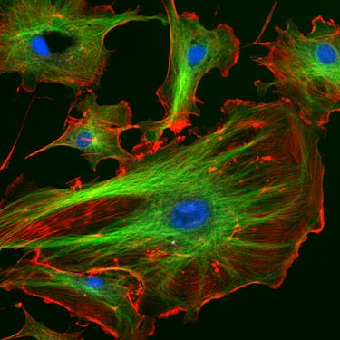
Endothelial cells under the fluorescence microscope. The microtubules are green (with FITC- labeled antibody), actin filaments are red (with phalloidin - TRITC ). The DNA in the cell nuclei was stained with DAPI (blue).
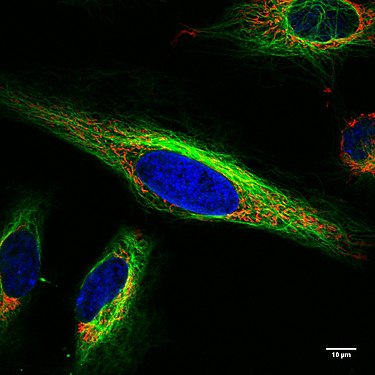
Living HeLa cells under the confocal microscope. Mitochondria in red, the cell nucleus in blue, microtubules in green.

Cell at the end of mitosis in telophase . Chromosomes blue (DAPI), microtubules red, the INCENP protein is colored green through a fusion with GFP.

Immunofluorescence image in the rat spinal ganglion . Two different proteins were stained with red or green fluorescent markers.

Metaphase chromosomes from a female human lymphocyte stained with Chromomycin A3.
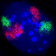
Cell nucleus of a mouse fibroblast , the territories of chromosomes 2 (red) and 9 (green) were stained by fluorescence in situ hybridization. DNA counterstaining in blue.
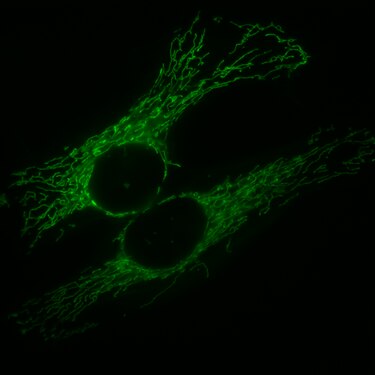
HeLa cells, the mitochondria, are marked with GFP, which is fused with a corresponding signal peptide .
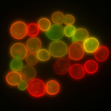
Yeast cells in which two different membrane proteins are fused with GFP or RFP (red fluorescent protein). Individual cells have different amounts of the two proteins and therefore different shades.


Applications in materials science
In contrast to the life sciences, fluorescent dyes are rarely used in materials science . The use of fluorescence microscopy is mostly limited to cases in which the material is autofluorescent. For example, some components of composite materials are fluorescent and can be distinguished from other non-fluorescent components. For a better representation of the situation, fluorescence can be combined with reflection in a confocal microscope . This means that fluorescent binders (base polymer) can be distinguished from non-fluorescent fibers in fiberglass- reinforced composite materials , for example .
Organic fibers in paper , wood or bast have been investigated in a number of studies to determine their arrangement or composition.
Different types of solar cells can also be examined using a fluorescence microscope. Confocal fluorescence microscopy is often used, also in combination with confocal reflection microscopy. In organic solar cells , the loss of fluorescent organic components caused by oxidation with oxygen that has entered the cell can be investigated; provided the breakdown products are not fluorescent. The influence of light on the formation of the perovskite layer of the same name was analyzed in perovskite solar cells .

Although many minerals fluoresce, fluorescence microscopy is little used in petrology . A notable exception is studies of coal and of organic inclusions in sediments . Pure minerals are usually not fluorescent, but fluorescence can be caused by various inorganic or organic impurities. Such rock-forming components of coal that have an organic origin are called macerals . A subgroup are the lipid-rich liptinites. These fluorescent components can be distinguished microscopically from non-fluorescent inorganic components particularly well on polished surfaces . During coal formation, the fluorescent properties change, so that materials from different deposits can be distinguished.
Special fluorescence microscopic procedures
Light disk microscopy

In the light sheet fluorescence microscopy ( English light sheet microscopy ; also light sheet microscopy or single plane illumination microscopy , SPIM) is the excitation light from the side as a lens or light sheet irradiated. This can be done using a second objective or a corresponding cylindrical lens that is perpendicular to the observation objective and illuminates a narrowly delimited plane of the specimen. Fluorescence is only generated in this illuminated pane and this plane is brought into focus in the observation lens. In other planes, therefore, no fuzzy background fluorescence is generated, which would lead to a reduction in the contrast in normal fluorescence microscopy. The method makes it possible to improve the axial resolution of a normal fluorescence microscope if the light sheet is thinner than the depth of field of the observation lens. The side lighting of the examination object is similar to the arrangement in the slit ultramicroscope .
Confocal and two-photon fluorescence microscopy

With confocal as well as two-photon microscopes, the specimen is scanned: the excitation light is focused on a point, the fluorescence from this point reaches the detector. The point is moved over the specimen and the fluorescence intensities measured in each case are combined to form an image in a control computer.
In confocal fluorescence microscopy, fluorescence is also produced in the illumination cone above and below the plane of focus. However, this does not reach the detector because it is blocked by a pinhole in the intermediate image plane. By blocking this background fluorescence, the signal emerges better in the focal plane compared to the background than in classical fluorescence microscopy. Because of these clearly higher contrast images, confocal microscopes are widely used in biological research.
A fluorescent dye can also be excited by two-photon absorption instead of by absorption of one photon . The prerequisite for this is that these two photons arrive at the fluorescent dye almost simultaneously, and that both together have the right energy content to raise an electron of the dye to an excited energy level. Both conditions can be met if a pulsed laser is used for excitation , which, depending on the fluorescent dye to be excited , generates wavelengths between 700 and 1200 nm with high intensity, and this light is focused on a point by the objective. The photon density is then so high that there is a sufficient probability that two photons will arrive at the fluorescent molecule at the same time. In contrast to confocal microscopy, where the readout volume is limited, the excitation volume is limited here. Longer-wave light penetrates biological tissue to a greater extent, as it is less strongly absorbed by these and also less strongly scattered . Two-photon fluorescence microscopy is therefore used to penetrate deeper into tissue than is possible with other methods. Along with methods that do not rely on fluorescence, this technique is called multiphoton microscopy or non-linear microscopy.
Fluorescence correlation spectroscopy

The fluorescence correlation spectroscopy (abbreviated FCS for English fluorescence correlation spectroscopy ) is a fluorescence microscopic method, but with it no image is generated. In a confocal microscope, the excitation laser is not scanned over the specimen, but parked in one place. A very small volume is thus observed over a longer period of time. If fluorescent molecules move into or out of this volume, the measured brightness changes. Such a series of measurements can be used, for example, to determine how quickly molecules diffuse in a solution . Since the diffusion speed depends, among other things, on the size, it is possible, for example, to investigate whether a fluorescence-labeled protein binds to a second protein, which is also present in the solution, and thus moves more slowly.
Process with increased resolution
In microscopy, resolution is the distance that two structures must have in order to be perceived as separate structures. Ernst Abbe was the first to understand in the 19th century that this resolution is fundamentally limited by diffraction . This limit is therefore called the Abbe limit. It can be calculated precisely using the appropriate formulas and, for good microscopes using oil immersion and depending on the wavelength, is around 200 nm.
The Abbe limit has long been considered insurmountable. From the second half of the 20th century, however, some microscopic methods were developed whose resolution is better than predicted by the Abbe limit. By far the oldest of these methods is confocal microscopy (see also the section on resolution in the article Confocal microscope.) The theoretical improvement, however, is only with the factor root of 2 ≈ 1.41. For practical reasons this cannot be reached either.

In the 1980s, which was TIRF microscopy ( English total internal reflection fluorescence microscopy suggested). It only stimulates fluorescent dyes in the specimen that are very close to the cover slip. If the preparation, for example living cells, is in an aqueous medium, the excitation from the cover slip penetrates only into a layer 100-200 nm thick. The layer thickness is thus significantly less than would be possible with normal microscopy due to diffraction. This results in a significantly higher contrast since only a small amount of material is excited to fluoresce. This special form of excitation is achieved by illuminating the specimen at an angle that is so large that total reflection occurs at the edge from the cover slip to the aqueous medium and the light beam does not penetrate the specimen at all. However, an evanescent wave occurs at the edge, which can lead to excitation, but which weakens very quickly with increasing distance from the cover slip.
While "resolution" by definition means the minimum distance between two structures, the exact position of an object can be measured very precisely. Fluorescence microscopy can therefore circumvent the Abbe limit by determining the exact position of objects in different color channels and then measuring the distance between them. This technique was developed in the 1990s and later referred to as Spectral Precision Distance Microscopy (SPDM). It can be used to measure distances between small fluorescent structures with an accuracy of about 70 nm. However, it does not lead to a general improvement in resolution, since each of the recorded color channels is subject to diffraction.
At the end of the 20th and the beginning of the 21st century, however, a number of methods were developed with which a general improvement is possible. They are collectively referred to in English as superresolution microscopy , sometimes also as nanoscopy . What they all have in common is that they are based on fluorescence microscopy. Three of these methods have gained some popularity and are commercially available: STED, structured illumination, and localization microscopy. There are also other methods that could not hold their own against the aforementioned, or that have only been used by individual groups so far. Some procedures are grouped together as RESOLFT microscopy due to their common properties .
High-resolution fluorescence microscopy was named Method of the Year 2008 by the journal Nature Methods . William Moerner , Eric Betzig, and Stefan Hell received the 2014 Nobel Prize in Chemistry for developing some of these methods.
STED microscopy

In the STED microscopy ( English stimulated emission depletion ) is diffraction limit significantly overcome. The excitation of a diffraction-limited volume in the specimen is followed by a ring-shaped de-excitation by light of longer wavelength. The excited molecules in the de-excitation area fall back into the ground state via stimulated emission . The volume emitting fluorescence is thereby significantly reduced and the resolution of the microscope is increased.
Structured lighting

With structured illumination or 3D-SIM microscopy (English structured illumination microscopy ), not all fluorochromes are excited, but only part of the preparation in the form of a certain 'structure', a striped pattern. When the known illumination pattern is superimposed on the unknown fluorochrome distribution in the specimen, moiré effects arise , the size of which is greater than the resolution limit, even if the unknown structure is smaller. By shifting and rotating the lighting pattern, the additional information from the moiré patterns of the respective images can be used to generate a final image with up to twice the resolution by computer calculation.
Localization microscopy
As localization microscopy (English localization microscopy ) are combined microscopic methods based on a common basic principle: while listening to classical fluorescence microscopy all fluorochromes are excited simultaneously, they are excited here one after the other, so that only a small part is illuminated by them. Many pictures are taken one after the other from one level of focus, often over a thousand. The exact position of the glowing fluorochromes is now determined in each of these images and this position is transferred to the final image. The processes differ in the method of how the individual dye molecules are switched on and off, ie made to “blink”.
The photoactivated localization microscopy (PALM) is based on variants of the green fluorescent protein , the one with light of certain wavelengths and let off. STORM and dSTORM use suitable fluorescent dyes which only rarely fluoresce in certain buffer solutions. Ground State Depletion (GSD) is based on the fact that at any point in time the majority of the fluorochromes are in a non-fluorescent triplet state that can be generated by strong light excitation. DNA-Paint is based on the temporary binding of short, single-stranded DNA molecules to complementary target molecules.
Further methods for improving the resolution
4Pi microscopy was the first commercially available superresolution technique, but is no longer available today. Another technology is Vertico-SMI , which was developed in Heidelberg.
Fluorescence Lifetime Microscopy (FLIM)
After excitation, a fluorescent substance remains in the excited state for a short period of time before it emits the fluorescent light. The duration of this period of time varies for a specific substance within a certain range, so that an average fluorescence lifetime can be determined for a particular substance. It is in the nanosecond range, for example for fluorescein at 3.25 ns, for Texas Red at 3.41 ns and for eosin at 1.1 ns. If the fluorescence excitation in the microscopic preparation is carried out with a pulsed or modulated laser and special detectors are used, then the time span after which the fluorescence arrives at the detector can be determined by means of special measuring methods . Fluorescent dyes can therefore be distinguished from one another not only by their color, but also by their lifetime. This is in the fluorescence lifetime microscopy (English fluorescence lifetime imaging microscopy , FLIM) exploited. There are pulsed and modulated lasers in the visible wavelength range for excitation with a photon. However, FLIM can also be used in combination with multi-photon excitation (see above), for which pulsed lasers are required anyway.
Förster resonance energy transfer (FRET)

With Förster resonance energy transfer (sometimes also: fluorescence resonance energy transfer), the energy of an excited fluorescent dye, the donor, is not given off by fluorescence, but is transferred directly to another fluorescent dye (acceptor). This is possible if firstly the donor and acceptor are less than 10 nm apart and secondly the emission energy of the donor corresponds to the excitation energy of the acceptor. The emission spectrum of the donor must therefore overlap with the excitation spectrum of the acceptor. For example, a green fluorescent dye can serve as a donor for an orange fluorescent acceptor. Another example is the cyan fluorescent protein CFP as a donor for the yellow fluorescent protein YFP.
If FRET occurs, the donor does not emit any fluorescence despite the excitation of the donor; instead, the fluorescence of the acceptor can be observed. The FRET efficiency decreases with the sixth power of the distance between donor and acceptor. The occurrence of FRET therefore indicates the direct proximity of the two, with an accuracy that is well below the limit of resolution.
Intentional bleaching for diffusion measurement (FRAP and FLIP)
With FRAP ( fluorescence recovery after photobleaching ), a fluorescence-labeled molecule in a living cell is intentionally bleached in a part of the cell by short-term, strong exposure to light, usually by means of a focused laser beam. It is then observed how quickly molecules from the non-bleached part of the cell return to the bleached part. Conclusions about the binding behavior of the molecule can be drawn from the determined diffusion speed.
With FLIP ( fluorescence loss in photobleaching ), on the other hand, an area of the cell is continuously bleached. It is observed how quickly the fluorescence decreases in the non-bleached part of the cell.
history
1904: Köhler's discovery
The first fluorescence microscopic observations were accidental and a nuisance. August Köhler , employee at the microscope manufacturer Carl Zeiss , wanted to increase the light microscopic resolution. The resolution depends on the wavelength, so he built a microscope for UV light to use its shorter wavelength. The image thus generated was not visible to the eyes, but could be captured photographically. He found that
“The object itself fluoresces under the influence of the ultraviolet radiation striking it. Such fluorescence occurs in the majority of the specimens. ... The fluorescent light ... is in any case partly in the visible range of the spectrum; ... It is obvious that this makes it more difficult, if not impossible, to perceive the image generated by the ultraviolet rays, which is actually important. ... Under certain circumstances, of course, the observation of this direct image could also offer interest ... "
So Köhler was aware early on that the fluorescence, which is disruptive in UV microscopy, could also enable useful applications.
1910–1913: First fluorescence microscopes and applications

The first commercially available fluorescence microscope was developed by Oskar Heimstädt , who headed the computing and design office at the Viennese microscope maker Karl Reichert . It was presented by Reichert personally in 1911 at the meeting of German naturalists and doctors . In the same year Heimstädt published a work with the title "The fluorescence microscope" in the journal for scientific microscopy.
UV light was well suited for fluorescence excitation as it was not visible to the eye and therefore no blocking filter was required. A good suggestion required that no visible UV light from the light source but as much UV light as possible reached the specimen. A suitable excitation filter was developed shortly beforehand, in 1910, by Hans Lehmann at Zeiss. It consisted of a filter cuvette which consisted of two chambers along the optical axis. The three walls were made of Jena blue uviol glass , one chamber was filled with saturated copper sulfate solution, the other with dilute nitrosodimethylaniline solution. The excitation light generated in this way was referred to as “filtered ultraviolet”. Since normal glass absorbs UV light, a quartz condenser was used a little later in order to obtain high illuminance levels. However, a new problem arose: the glass lenses in the objective began to fluoresce. Lehmann therefore used a dark-field condenser : the excitation light was guided past the lens and residues of visible light from the light source in the microscopic image were also avoided.
Heimstädt wrote about the possibilities and future prospects of fluorescence microscopy
"It is Z. For example, it is easy to detect the presence of very small amounts of ergot in the flour ... because starch fluoresces intensely purple, while ergot emits a yellowish white light. ...
Whether and how far the fluorescence microscope ... [includes] a possibility of expanding the microscopic imaging area, the future must teach. "
Also in 1911 Michail Tswett described the fluorescence of the chloroplasts. In 1913, Stanislaus von Prowazek published the first work in which fluorescent dyes were used, namely eosin and neutral red .
One year after Reichert's fluorescence microscope, the Zeiss “luminescence microscope” developed by Lehmann was presented at the meeting of German naturalists and doctors in 1912. Dark field illumination leads to a reduced numerical aperture and thus to a reduced resolution. Lehmann therefore opted for normal bright field lighting with UV light. To prevent UV light from getting into the eye, he put on a UV-blocking glass filter made of Euphos glass, which was used as a cover slip . The filter had to be between the preparation and the objective in order to avoid fluorescence excitation in the objective, so no other position for the filter was possible. The condenser had quartz lenses, the microscope slides used were made of rock crystal to ensure UV transmission. The recommended standard magnification was 62 × (including eyepiece magnification), 300 × should not be exceeded. The additional fluorescence equipment, i.e. without the actual microscope, cost around 500 marks with the cheapest excitation light source, a manually adjustable arc lamp . There was also 4.50 M for a 0.5 mm thick 30 × 25 mm rock crystal slide and one mark per Euphos glass cover slip. In addition to black and white photographs, color images could also be created using the autochrome process.
1933–1940: Max Haitinger and fluorochroming

In the early days of fluorescence microscopy, autofluorescent objects were examined almost exclusively. Even Max Haitinger first private researchers in Weidling near Vienna and later at the University of Vienna , began by studying the fluorescence of wine and fruit wines. From 1933, however, he developed fluorescent stains, which he called "fluorochromes". The terms secondary fluorescence for signals to be generated and primary fluorescence for those naturally present in the preparation come from him. He also introduced the term fluorochrome for a fluorescent dye. He first used plant extracts as fluorochromes and later a number of chemicals. This enabled him to stain thin sections of animal and human tissues, so that histologists also began to be interested in fluorescence microscopy. Since only very low concentrations of the fluorochromes were required, live stains were also possible, which were mainly used in botany. With auramine O staining of managed tuberculosis bacteria. Multiple staining was also possible. Haitinger published a first paper in 1934, his book "Fluorescenzmikoskopie - Your application in histology and chemistry" was published in 1938.
Haitinger worked closely with the Reichert company to improve their fluorescence microscope. The new model "Kam F" was sold from 1931. This too had an arc lamp with iron electrodes as the light source, as this had a comparatively high UV component between 300 nm and 400 nm. Nevertheless, he needed up to 20 minutes exposure time for his photographs. For low magnifications, he mentions exposure times with carbon arc lamps of one to ten minutes. The nitrosyldimethylaniline solution in the excitation filter cuvette could be replaced by black glass filters containing nickel oxide. The copper sulphate solution, which filtered the remaining red component in the excitation light, was only replaced by blue glass filters in the early 1940s. The lighting was carried out by a bright field condenser with normal glass; it was found that quartz glass is not required for this. The remaining excitation light was blocked at the eyepiece by attaching a blocking filter made of 1 mm thick yellow glass. If a colorless barrier filter was required, a cuvette with a 5 mm thick layer of sodium nitrite solution could be used instead. Cover glasses made of Euphos glass were no longer necessary thanks to the yellow blocking filter, and it was also shown that normal microscope slides were suitable. This reduced the running costs considerably.

In his book from 1938, Haitinger also describes incident light illuminations for fluorescence microscopy of opaque objects (Epicondensor from Zeiss-Jena, Epilum from Optical Works C. Reichert-Wien (see schematic drawing), Ultropak from E. Leitz-Wetzlar and Univertor from E. Busch-Rathenow ). However, they cannot be compared with today's incident-light fluorescence excitation using a dichroic beam splitter. As application examples, he cites the examination of food, drugs and dyes as well as initial examinations of preparations from which thin sections are to be made. He describes incident light illuminations for studies on living animals as "particularly valuable".
Around 1940 Osram brought super- high pressure mercury lamps onto the market, for which lighting devices were soon added to the range at Zeiss and, with Haitinger's co-development, at Reichert (Lux UV and Lux UW). In addition to the significantly simplified handling and greater brightness, these lamps not only emit individual lines, but a continuous spectrum with which all fluorescent substances can be excited. Nor did they produce unpleasant fumes like iron arc lamps. Similar lamps are still in use today.
In the 1940s, color slide film began to gain acceptance for documentation purposes. Despite all the progress, the exposure times were mostly still in the two-digit minute range.
1942–1958: Development of immunofluorescence and the fluorescence of conventional dyes
A breakthrough for fluorescence microscopy was the introduction of immunofluorescence . 1942 published Albert Coons and colleagues coupling of fluorescein - isocyanate to antibodies . With its bright green fluorescence, this fluorochrome stood out better from the bluish autofluorescence of many tissues than the previously tried anthracene isocyanate. The antibodies were directed against pneumococci , which could be detected in mouse tissues by fluorescence microscopy. However, coupling the antibodies was technically demanding and the conjugates were unstable.
Siegfried Strugger noted that some known conventional dyes also fluoresce, such as neutral red and rhodamine B . He also introduced acridine orange to fluorescence microscopy. In a book in 1949 he described in detail the possibilities of fluorescence excitation with blue light instead of UV. Strugger used incident light to track the flow of water in plants.
In 1958, JL Riggs and colleagues achieved a significant improvement in immunofluorescence by using isothiocyanates instead of isocyanates. Another working group had in the meantime succeeded in detecting two colors with fluorescein isocyanate and the orange fluorescent rhodamine B isocyanate. Riggs and his colleagues have now succeeded in labeling antibodies with the much more stable fluorescein isothiocyanate (FITC) and rhodamine B isothiocyanate.
1962–1972: Johan Sebastiaan Ploem and the introduction of the interference filter
In the 1950s, fluorescence microscopy was only performed with UV, violet or blue excitation light. This only changed with the introduction of interference filters in the 1960s, driven by the Dutchman Johan Sebastiaan Ploem . The first to use a dichroic beam splitter in microscopy were the Russians Brumberg and Krylova in 1953. However, the work, published in Russian, remained unknown in the West and was only "rediscovered" later.
Driven by the development of numerous antibodies for immunofluorescence, there was a need for fluorochromes of different colors. However, these are often difficult to stimulate through conventional use with UV light. Around 1962, Ploem began working with the Schott works in Mainz to develop dichroic beam splitters that reflected blue or green light. Schott had previously manufactured many of the glass filters commonly used in fluorescence microscopy. The Leitz company supplied Ploem with an opaque incident light with a semi-transparent, color-independent mirror. This was rebuilt at the Universiteit van Amsterdam and received a slide with four positions for dichroic beam splitters for excitation with UV, violet, blue and green, so that the respective excitation wavelength could be conveniently selected. For the first time, the excitation came through the lens, as is usual today. By choosing narrow-band interference filters for blue or green excitation light, the dyes FITC (green fluorescent) and tetramethylrhodamine isothiocyanate (TRITC; orange fluorescent), which are frequently used in immunofluorescence, can be excited close to their absorption maximum without simultaneously having large amounts of autofluorescence due to unnecessary excitation wavelengths trigger. Ploem published his results in several papers starting in 1965.

Leitz then developed the PLOEMOPAK, a device on which four beam splitters could be rotated alternately into the beam path. Later versions were supplemented with blocking filters and excitation filters until a variant finally came onto the market around 1972 that contained four fluorescence filter cubes each with an excitation filter, beam splitter and blocking filter. The user could exchange the cubes to adapt them to the fluorochromes used.
With this the development of the epifluorescence microscope, as it is still used today, was in principle complete. However, it would take several years before this type of construction became generally accepted. British microscopy textbooks from 1975 and 1977 only mention the possibility of UV excitation and transmitted light illumination. A later one from 1982 said that the lighting is usually done with a dark field condenser, but also described incident light lighting with a dichroic beam splitter and presented it as the more light-sensitive one. The possibility of being able to detect fluorochromes such as FITC and rhodamine one after the other by replacing all filters was also mentioned.
A West German textbook from 1985 described all three possibilities, transmitted light bright and dark field and reflected light bright field excitation through the lens, attributed the latter to a particularly simple setting (since no condenser is required) and high excitation intensity with excellent contrast, and mentioned the option of filter blocks to exchange quickly. Leitz, Olympus , Reichert, Zeiss and Jena were named as manufacturers of such systems , which probably meant VEB Carl Zeiss Jena . A textbook from 1988 mentioned the older methods, but then stated: “Modern fluorescence microscopes work according to the principle of reflected light brightfield excitation” with a dichroic divider plate. It was further stated: "Most microscope manufacturers offer equipment for transmitted light and reflected light fluorescence microscopy".
Web links
- Michael Volger (Ed .: Irene K. Lichtscheidl): Fluorescence microscopy. Retrieved on March 25, 2017 (theoretical introduction and instructions for practical application at the University of Vienna. Univie.ac.at (PDF)).
- Multi-Wavelength Epi-Illumination in Fluorescence Microscopy by Johan Sebastiaan Ploem and Friedrich Walter on Leica Science Lab.
- Fluorescent dye databases: Fluorophores.org , Spectra Database at the University of Arizona, Fluorescence SpectraViewer at Thermo Fisher.
Individual evidence
- ↑ a b Jörg Haus: Optical microscopy . Wiley-VCH, Weinheim 2014, ISBN 978-3-527-41127-6 , pp. 163-173 .
- ↑ a b c d e f g h i j k l m Guy Cox: Optical Imaging Techniques in Cell Biology . Second ed.CRC Press, Taylor & Francis Group, Boca Raton, FL, USA 2012, ISBN 978-1-4398-4825-8 , pp. 35-48 .
- ^ Markus Axmann, Josef Madl, Gerhard J. Schütz: Single-Molecule Microscopy in the Life Sciences . In: Ulrich Kubitscheck (Ed.): Fluorescence Microscopy . Wiley-Blackwell, Weinheim 2013, ISBN 978-3-527-32922-9 , pp. 293–343, here p. 309 .
- ↑ I. Georgakoudi, BC Jacobson, MG Müller, EE Sheets, K. Badizadegan, DL Carr-Locke, CP Crum, CW Boone, RR Dasari, J. Van Dam, MS field: NAD (P) H and collagen as in vivo quantitative fluorescent biomarkers of epithelial precancerous changes. In: Cancer research . Volume 62, Number 3, February 2002, pp. 682-687, PMID 11830520 .
- ^ MR Speicher, S. Gwyn Ballard, DC Ward: Karyotyping human chromosomes by combinatorial multi-fluor FISH. In: Nature genetics . Volume 12, Number 4, April 1996, pp. 368-375, doi: 10.1038 / ng0496-368 . PMID 8630489 .
- ↑ A. Bolzer, G. Kreth, I. Solovei, D. Koehler, K. Saracoglu, C. Fauth, S. Müller, R. Eils, C. Cremer, MR Speicher, T. Cremer: Three-dimensional maps of all chromosomes in human male fibroblast nuclei and prometaphase rosettes. In: PLoS biology . Volume 3, number 5, May 2005, p. E157, doi: 10.1371 / journal.pbio.0030157 . PMID 15839726 , PMC 1084335 (free full text).
- ^ A b Douglas B. Murphy, Michael W. Davidson: Fundamentals of Light Microscopy and Electronic Imaging . Second ed. Wiley-Blackwell, Hoboken, NJ, USA 2013, ISBN 978-0-471-69214-0 , pp. 45-50 .
- ↑ Guy Cox: Optical Imaging Techniques in Cell Biology . Second ed.CRC Press, Taylor & Francis Group, Boca Raton, FL, USA 2012, ISBN 978-1-4398-4825-8 , pp. 75-81 .
- ^ Douglas B. Murphy, Michael W. Davidson: Fundamentals of Light Microscopy and Electronic Imaging . Second ed. Wiley-Blackwell, Hoboken, NJ, USA 2013, ISBN 978-0-471-69214-0 , pp. 389-413 .
- ^ Rolf Theodor Borlinghaus: Confocal microscopy in white: optical sections in all colors . Springer Spectrum, 2016, ISBN 978-3-662-49358-8 .
- ^ Ian D. Johnson: Practical Considerations in the Selection and Application of Fluorescent Probes . In: James Pawley (Ed.): Handbook of Biological Confocal Microscopy . 3. Edition. Springer Science and Business Media LLC, 2006, ISBN 0-387-25921-X , Chapter 1, pp. 353-367 .
- ^ A b Douglas B. Murphy, Michael W. Davidson: Fundamentals of Light Microscopy and Electronic Imaging . Second ed. Wiley-Blackwell, Hoboken, NJ, USA 2013, ISBN 978-0-471-69214-0 , pp. 361-365 .
- ↑ a b c Gerd Ulrich Nienhaus, Karin Nienhaus: Fluorescence Labeling . In: Ulrich Kubitscheck (Ed.): Fluorescence Microscopy . Wiley-Blackwell, Weinheim 2013, ISBN 978-3-527-32922-9 , pp. 143-173, here pp. 147-148 .
- ^ Douglas B. Murphy, Michael W. Davidson: Fundamentals of Light Microscopy and Electronic Imaging . Second ed. Wiley-Blackwell, Hoboken, NJ, USA 2013, ISBN 978-0-471-69214-0 , pp. 227 f .
- ^ A b Guy Cox: Optical Imaging Techniques in Cell Biology . Second ed.CRC Press, Taylor & Francis Group, Boca Raton, FL, USA 2012, ISBN 978-1-4398-4825-8 , pp. 181-190 .
- ↑ Guy Cox: Optical Imaging Techniques in Cell Biology . Second ed.CRC Press, Taylor & Francis Group, Boca Raton, FL, USA 2012, ISBN 978-1-4398-4825-8 , pp. 169-180 .
- ^ Douglas B. Murphy, Michael W. Davidson: Fundamentals of Light Microscopy and Electronic Imaging . Second ed. Wiley-Blackwell, Hoboken, NJ, USA 2013, ISBN 978-0-471-69214-0 , pp. 167 .
- ^ Ashley R. Clarke, Colin Nigel Eberhardt: Microscopy Techniques for Materials Science . Woodhead Publishing, Abington Hall 2002, ISBN 978-1-85573-587-3 , pp. 255, 279-284 .
- ^ LA Donaldson: Analysis of fibers using microscopy . In: Handbook of Textile Fiber Structure. Fundamentals and Manufactured Polymer Fibers. Volume 1 in Woodhead Publishing Series in Textiles . 2018 Elsevier, 2009, p. 121–153 , doi : 10.1533 / 9781845696504.1.121 ( excerpt ).
- ^ Pankaj Kumar: Organic Solar Cells: Device Physics, Processing, Degradation, and Prevention . CRC Press, 2016, ISBN 978-1-4987-2327-5 , pp. 23 ( Google Books ).
- ↑ JH Huang, FC Chien, P. Chen, KC Ho, CW Chu: Monitoring the 3D nanostructures of bulk heterojunction polymer solar cells using confocal lifetime imaging. In: Analytical Chemistry . Volume 82, Number 5, March 2010, pp. 1669–1673, doi: 10.1021 / ac901992c , PMID 20143827 .
- ↑ A. Ummadisingu, L. Steier, JY Seo, T. Matsui, A. Abate, W. Tress, M. Grätzel: The effect of illumination on the formation of metal halide perovskite films. In: Nature . Volume 545, number 7653, 05 2017, pp. 208-212, doi: 10.1038 / nature22072 , PMID 28445459 .
- ^ FWD Rost: Fluorescence Microscopy Volume II . Cambridge University Press, 1995, ISBN 978-0-521-41088-5 , pp. 40–47 ( online at Google Books ).
- ↑ a b c d e Jörg Haus: Optical microscopy . Wiley-VCH, Weinheim 2014, ISBN 978-3-527-41127-6 , pp. 189-200 .
- ↑ Guy Cox: Optical Imaging Techniques in Cell Biology . Second ed.CRC Press, Taylor & Francis Group, Boca Raton, FL, USA 2012, ISBN 978-1-4398-4825-8 , pp. 63 ff .
- ↑ Guy Cox: Optical Imaging Techniques in Cell Biology . Second ed.CRC Press, Taylor & Francis Group, Boca Raton, FL, USA 2012, ISBN 978-1-4398-4825-8 , pp. 109 ff .
- ↑ Guy Cox: Optical Imaging Techniques in Cell Biology . Second ed.CRC Press, Taylor & Francis Group, Boca Raton, FL, USA 2012, ISBN 978-1-4398-4825-8 , pp. 223 ff .
- ↑ Harald Bornfleth, Kurt Satzler, Roland Eils, Christoph Cremer: High-precision distance measurements and volume-conserving segmentation of objects near and below the resolution limit in three-dimensional confocal fluorescence microscopy . In: Journal of Microscopy . tape 189 , no. 2 , February 1998, p. 118 , doi : 10.1046 / j.1365-2818.1998.00276.x .
- ↑ Steffen Dietzel, Roland Eils, Kurt Sätzler, Harald Bornfleth, Anna Jauch, Christoph Cremer, Thomas Cremer: Evidence against a Looped Structure of the Inactive Human X-Chromosome Territory . In: Experimental Cell Research . tape 240 , no. 2 , May 1998, pp. 187 , doi : 10.1006 / excr.1998.3934 , PMID 9596991 .
- ↑ Anonymous: Method of the Year 2008. In: Nature Methods . 6, 2009, p. 1, doi: 10.1038 / nmeth.f.244 .
- ↑ Volker Westphal, Silvio O. Rizzoli, Marcel A. Lauterbach, Dirk Kamin, Reinhard Jahn, Stefan W. Hell : Video-Rate Far-Field Optical Nanoscopy Dissects Synaptic Vesicle Movement . In: Science . tape 320 , no. 5873 , April 11, 2008, p. 246-249 , doi : 10.1126 / science.1154228 .
- ↑ Guy Cox: Optical Imaging Techniques in Cell Biology . Second ed.CRC Press, Taylor & Francis Group, Boca Raton, FL, USA 2012, ISBN 978-1-4398-4825-8 , pp. 245-247 .
- ↑ Guy Cox: Optical Imaging Techniques in Cell Biology . Second ed.CRC Press, Taylor & Francis Group, Boca Raton, FL, USA 2012, ISBN 978-1-4398-4825-8 , pp. 207 ff .
- ^ Douglas B. Murphy, Michael W. Davidson: Fundamentals of Light Microscopy and Electronic Imaging . Second ed. Wiley-Blackwell, Hoboken, NJ, USA 2013, ISBN 978-0-471-69214-0 , pp. 280 ff .
- ^ A b Guy Cox: Optical Imaging Techniques in Cell Biology . Second ed.CRC Press, Taylor & Francis Group, Boca Raton, FL, USA 2012, ISBN 978-1-4398-4825-8 , pp. 213 ff .
- ^ A b Guy Cox: Optical Imaging Techniques in Cell Biology . Second ed.CRC Press, Taylor & Francis Group, Boca Raton, FL, USA 2012, ISBN 978-1-4398-4825-8 , pp. 201 ff .
- ↑ a b c d e f g h i j k l Dieter Gerlach: History of microscopy . Verlag Harri Deutsch, Frankfurt am Main 2009, ISBN 978-3-8171-1781-9 , pp. 625-657 .
- ↑ a b c Oskar Heimstädt: The fluorescence microscope . In: Journal of Scientific Microscopy . tape 28 , 1911, pp. 330-337 ( online ).
- ↑ a b c Fritz Bräutigam, Alfred Grabner: Fluoreszenzmikoskopie . In: Fritz Bräutigam, Alfred Grabner (ed.): Contributions to fluorescence microscopy (= 1st special volume of the journal "Microscopy" ). Verlag Georg Fromme & Co., Vienna 1949, p. 25-34 .
- ↑ Michail Tswett: About Reichert's fluorescence microscope and some observations made with it about chlorophyll and cyanophyll. In: Reports of the German Botanical Society . Volume 29, 1911, pp. 744-746. ( online - quoted from Gerlach, 2009.)
- ^ Stanislaus von Prowazek: Fluorescence of the cells. - Reicherts fluorescence microscope. In: Zoologischer Anzeiger . Volume 42, 1913, pp. 374-380. ( online - quoted from Gerlach, 2009.)
- ↑ a b c d Max Haitinger: Fluorescence microscopy - your application in histology and chemistry . Academic Publishing Company, Leipzig 1938.
- ^ Karl Höfler : Max Haitinger 1868-1946 . In: Hugo Freund, Alexander Berg (Hrsg.): Applied natural sciences and technology (= history of microscopy, life and work of great researchers . Volume III ). Umschau Verlag, Frankfurt am Main 1966, p. 187-194 .
- ^ Albert H. Coons, Hugh J. Creech, R. Norman Jones, Ernst Berliner: The Demonstration of Pneumococcal Antigen in Tissues by the Use of Fluorescent Antibody . In: J Immunol . tape 45 , no. 3 , November 1, 1942, pp. 159-170 ( online ).
- ↑ JL Riggs, RJ Seiwald, JH Burckhalter, CM Downs, TG Metcalf: Isothiocyanate compounds as fluorescent labeling agents for immune serum. In: The American Journal of Pathology . Volume 34, Number 6, Nov-Dec 1958, pp. 1081-1097. PMID 13583098 , PMC 1934794 (free full text).
- ↑ ES Perner: The methods of fluorescence microscopy . In: Hugo Freund (Ed.): The optical fundamentals, the instruments and auxiliary devices for microscopy in technology. Part 1: General instruments of transmitted light microscopy (= manual of microscopy in technology . Volume 1 , part 1). Umschau Verlag, Frankfurt am Main 1957, p. 357-431, here p. 371 .
- ↑ Heinz Appelt: Introduction to microscopic examination methods . 4th edition. Academic publishing company Geest & Portig, Leipzig 1959, p. 283 .
- ↑ EM Brumberg, TN Krylova: O fluoreschentnykh microscopic opaque . In: Zh. obshch. biol. 14, 1953, p. 461.
- ↑ a b Johan Sebastiaan Ploem, Friedrich Walter: Multi-Wavelength Epi-Illumination in Fluorescence Microscopy . In: Leica Microsystems (Ed.): Scientific and Technical Information CDR . tape 5 , 2001, p. 1–16 ( online at the Leica Science Lab).
- ^ HN Southworth: Introduction to Modern Microscopy . Wykeham Publications LTD, a member of the Taylor & Francis Group, London 1975, ISBN 0-85109-470-8 , pp. 84-85 .
- ↑ W. Burrels: Microscope Technique. A Comprehensive Handbook for General and Applied Microscopy . New revised ed. Fountain Press, London 1977, ISBN 0-85242-511-2 , pp. 481-483 .
- ↑ Michael Spencer: Fundamentals of light microscopy (= IUPAB Biophysics Series . Volume 6 ). Cambridge University Press, Cambridge, England 1982, ISBN 0-521-28967-X , pp. 40-45 .
- ↑ Dieter Gerlach: The light microscope. An introduction to function and application in biology and medicine . 2nd Edition. Thieme Verlag, Stuttgart 1985, ISBN 3-13-530302-0 , p. 210-224 .
- ↑ Gerhard Göke: Modern methods of light microscopy: from the transmitted light bright field to the laser microscope . Franckh'sche Verlagshandlung, Stuttgart 1988, ISBN 3-440-05765-8 , p. 211-212 .