
Carbon dioxide in the earth's atmosphere


Carbon dioxide (CO 2 ) is a trace gas with a volume fraction of about 0.04% (about 400 ppm ) in the earth's atmosphere . The mass fraction is about 0.06%.
Despite its low concentration, carbon dioxide is of elementary importance for life on earth in many ways: Plants absorb the trace gas they need and give off oxygen ( photosynthesis ), while most living things and many other natural processes breathe in and release carbon dioxide is released into the earth's atmosphere.
As a greenhouse gas , CO 2 has a major influence on the earth's climate through the greenhouse effect and, through its solubility in water, the pH value of the oceans. In the course of the earth's history , the atmospheric CO 2 content has fluctuated considerably and was often directly involved in a number of serious climate change events .
Carbon cycle

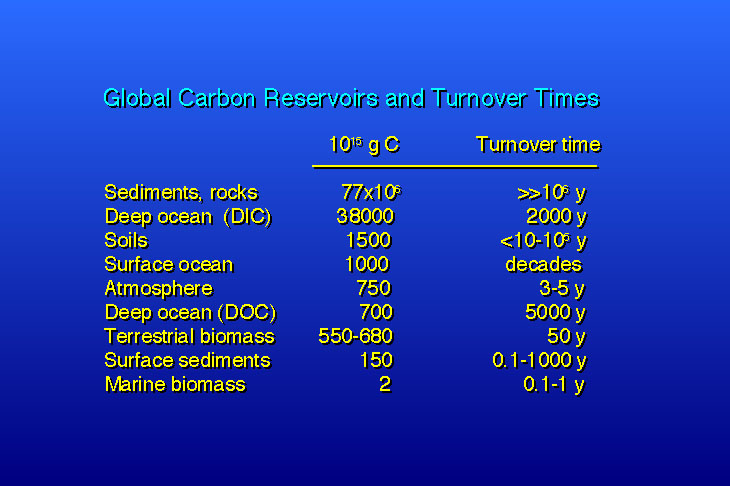
Around 65,500,000 gigatons of carbon are stored in the earth's crust . In 2008 there were around 3,000 gigatons of CO 2 in the earth's atmosphere . This corresponds to about 800 gigatons of carbon - about 0.0012 percent of the amount in the outer rock on earth.
In the carbon cycle , a very large amount of carbon is constantly transferred between the atmosphere and other depots such as B. Seas, creatures and soils exchanged. Most CO 2 sources are of natural origin and are offset by natural CO 2 sinks. The atmospheric carbon dioxide concentration is influenced by the metabolism of living beings on earth, but also by reactions that take place independently of any life and have their origin in physical and chemical processes. The time constant , i.e. H. the speed of these processes varies widely and ranges from a few hours to several millennia.
The carbon dioxide concentration of the young earth had its origin in volcanic activity, which continues to add carbon dioxide to the atmosphere and currently releases around 150 to 260 megatons of carbon dioxide annually. Since the earth's existence, trace gas has been removed from the atmosphere by weathering rock. Part of it is also deposited through biogenic sedimentation and thus withdrawn from the cycle.
These abiotic processes are countered by considerably larger material flows that originate from the breathing of living beings. The burning of organic material by forest fires is also one of the natural sources of carbon dioxide .
Since CO 2 dissolves well in water, a change in the concentration of this trace gas in the air also affects the carbonic acid content and thus the pH value of the world's seas and lakes . The rise in atmospheric carbon dioxide concentration since the beginning of the industrial revolution has therefore led to both ocean acidification - almost half of the carbon dioxide introduced into the atmosphere by humans went into solution in the world's oceans - and the acidification of freshwater lakes .
Interaction with plants

Plants convert carbon dioxide into sugar , especially glucose , with the help of photosynthesis . They gain the energy they need for this reaction from the absorption of sunlight by chlorophyll ; oxygen is produced as a waste product. This gas is released into the atmosphere by plants, where it is then used for the respiration of heterotrophic organisms and other plants; this creates a cycle . Through these material flows, the carbon dioxide in the atmosphere is completely exchanged every 3 to 5 years on average. Land plants prefer to take up the lighter carbon isotope 12 C. This effect can be measured with the help of isotope studies .
The natural decay of organic material in forests and grasslands as well as fires that recur in nature lead to an annual release of approx. 439 gigatons of carbon dioxide. New plant growth completely compensates for this effect, as it absorbs around 450 gigatons annually.
The pre-industrial concentration of 280 ppm, but also the currently significantly increased concentration of slightly over 400 ppm, is below the optimal value for ideal growth for C 3 plants . In greenhouses , the carbon dioxide content of the air is therefore artificially increased to values of 600 ppm and more. This carbon dioxide fertilization can increase plant growth by up to 40% under otherwise ideal conditions. In nature, however, such a high increase in growth through CO 2 fertilization is only to be expected where plant growth is not limited by a shortage of nutrients and / or water. Over the period from 1982 to 2010, a significant globally detectable effect of CO 2 fertilization was established. In addition, twice as much carbon dioxide was absorbed by the biosphere in 2010 than in 1960; however, man-made emissions quadrupled during this period. Although 90% of all plant species are C 3 plants, 40% of the earth's surface are colonized by C 4 plants , which is therefore of great ecological and economic importance. Similar to the CAM plants adapted to very dry and warm habitats , C 4 plants only react to CO 2 fertilization with an increase in growth of a few percent, since they were able to absorb the trace gas very well even in the pre-industrial atmospheric concentration.
Effects of climate change

The efficiency of the enzyme Rubisco, which is responsible for the photosynthesis of plants, depends on its temperature and the CO 2 concentration in the ambient air. Although the tolerance to higher temperatures also increases with increasing CO 2 concentration, it is to be expected that the global warming associated with the increase in the CO 2 content of the atmosphere will lead to a decrease in photosynthesis rate and thus a decrease in primary production in some plant species .
The influence of increased carbon dioxide concentration, which has so far been considered beneficial in some cultivated plants, was investigated with regard to the biosphere as part of the FACE experiment . The results - depending on the plant - varied.
Spatial and temporal fluctuations in atmospheric concentration

Since the metabolism of plants is directly dependent on light, ground-level CO 2 concentrations fluctuate during the day . With sufficient plant cover there is a maximum at night and a minimum during the day. In and around metropolitan areas, the CO 2 concentration is high, but in forests it is significantly lower than in the surrounding area. In some regions of South America and Africa, fluctuations of around 60 ppm occur during the day. In closed rooms, the concentration can increase up to ten times the average value of the mean concentration in the open air.
When looking at the course of the concentration over several years, an annual fluctuation of 3–9 ppmv can be seen, which is caused by the growing season of the northern hemisphere. The influence of the northern hemisphere dominates the annual cycle of fluctuations in the carbon dioxide concentration, because there are much larger land areas and thus a larger biomass than in the southern hemisphere. The concentration is highest in May in the Northern Hemisphere, as spring greening begins at this time; it reaches its minimum in October, when photosynthetic biomass is greatest.
Due to the temperature dependence of the plant metabolism, there is also a difference between the equatorial CO 2 concentrations and the data obtained in arctic latitudes; these show the seasonal influence of the growth period: while the annual variation of the curves close to the equator is only approx. 3 ppm, in arctic latitudes it is 20 ppm.
Charles Keeling pioneered the study of the carbon dioxide concentration in the earth's atmosphere . In the late 1950s, he not only described the above-mentioned oscillations for the first time, but was also able to use the Keeling curve he created to prove for the first time that humans increase the concentration of this trace gas.
Importance as a greenhouse gas

CO 2 is an important greenhouse gas : It absorbs and emits infrared radiation at wavelengths of 4.26 µm and 14.99 µm ( asymmetrical stretching or bending vibration ). When the sky is clear, CO 2 accounts for 26% of the total greenhouse effect .
60% of the greenhouse effect can be attributed to water vapor , but the concentration of water vapor in the earth's atmosphere depends solely on the global average temperature of the earth, i.e. on the vapor pressure , via the Clausius-Clapeyron equation , and can only be changed permanently by this. In this way, water vapor only has an intensifying effect on global temperature changes. This makes carbon dioxide the most important greenhouse gas, the concentration of which can be changed directly and permanently. The global warming potential of other trace gases is related to that of CO 2 .
Since the middle of the 19th century, the CO 2 concentration has increased due to human activities. A doubling of the atmospheric CO 2 concentration from the pre-industrial value from 280 ppm to 560 ppm would, according to the current state of science, probably lead to global warming of 3 ° C. This value is called climate sensitivity .
Course in the history of the earth

Life, but also abiotic processes, have always had a major influence on the carbon dioxide concentration in the earth's atmosphere, but these were also shaped by it. So there is a mutual relationship.
Control mechanism of the earth
In geological terms, the (mostly) primarily caused by carbon dioxide greenhouse effect was of decisive importance. On earth there was water in liquid form very early on. The paradox of the weak young sun describes how, in spite of a weak sun, increased temperatures came about on the young earth. The luminosity of the sun has increased by around 30% since its formation 4.6 billion years ago. This has to be considered against the background that doubling or halving the pre-industrial CO 2 concentration of 280 ppm causes the same change in radiative forcing as a change in the solar constant of 2%. The concentration of greenhouse gases - especially carbon dioxide and methane - has fluctuated strongly several times in the course of the earth's history, but has fallen sharply over the entire period as a result of a self-regulating mechanism. Increased temperature caused increased weathering of the earth's surface and the precipitation of carbon dioxide in the sea in the form of lime . As a result, the carbon dioxide content decreased, as a result of which the temperature decreased and weathering and precipitation decreased and the temperature subsequently leveled off again at the old value with a lower carbon dioxide content in the atmosphere.
During the Great Oxygen Catastrophe about 2.4 billion years ago, the weakening of the greenhouse effect was very rapid, as the strong greenhouse gas methane was oxidized on a large scale and consequently almost completely disappeared from the atmosphere. It is very likely that this process was the cause of the Paleoproterozoic glaciation , with a duration of 300 million years probably the longest Snowball Earth event in Earth's history. Much of the earth was covered with ice.
Volcanoes continued to emit greenhouse gases such as carbon dioxide during glaciation, which accumulated in the atmosphere due to the fact that weathering and precipitation in the sea no longer took place. The carbon dioxide content rose to extremely high levels over a period of around 10 million years until the greenhouse effect was strong enough to melt the ice. As a result, the earth's surface, which was now exposed again, absorbed significantly more sunlight, and a global sauna climate followed for some 10,000 years. Due to the now severe weathering and precipitation, the carbon dioxide content was greatly reduced and huge amounts of lime were deposited within a very short time, which ultimately led to a temperate climate again as before, but with significantly reduced methane and CO 2 content in the atmosphere. Ultimately, two abiotic climate regulators are responsible for the fact that the climate in geological periods has leveled off again and again despite the changed radiation output of the sun and environmental conditions changed by life itself at moderate temperatures: volcanism and plate tectonics as recycler of lime deposits and thus as carbon dioxide producers and weathering and precipitation as a carbon dioxide sink.
Precambrian (early earth period)
It is believed that after the formation of the earth 4.57 billion years ago, the first life forms already existed at a very early stage. Cyanobacteria and algae began to produce oxygen around 3.5 billion years ago in the Precambrian - for which they absorbed CO 2 .
The determination of the atmospheric carbon dioxide concentration hundreds of millions of years ago is carried out by evaluating various proxy data . As part of isotope studies are borates in the shells of foraminifera analyzed. In an acidic environment, 11 B is increasingly incorporated into boric acid , which is necessary for the structure of the shell of these living beings. This enables conclusions to be drawn about the prevailing pH value, including the carbonic acid content of seawater. The CO 2 concentration can also be determined with the aid of Δ13C , another isotope test. In the development of the earth's atmosphere it is assumed that the "first atmosphere" had a carbon dioxide content of approx. 10%. However, this assumption is fraught with great uncertainty.
Phanerozoic
In the wake of the Great Oxygen Disaster , the oxygen concentration increased significantly both in the oceans and in the atmosphere. The associated transition from anaerobic to aerobic , i.e. a metabolism that is not based on oxygen conversion, but on an oxidative, oxygen-based metabolism, probably resulted in a mass extinction of anaerobic organisms in the previously oxygen-free biotopes, but it also opened up evolution new ways, as by oxidation there is far more energy available for metabolic processes than anaerobic life forms can use. At the time of the Cambrian explosion , when the representatives of all animal phyla existed at that time emerged within 5 to 10 million years, the atmospheric CO 2 content was at a high level of over 0.6% (= 6000 ppm). In contrast, the oxygen content of the air envelope increased only very slowly and stagnated at around 3% in the further course of the Proterozoic . It was not until the beginning of the ancient world ( Paleozoic ) 541 million years ago that its concentration increased significantly. It first reached its current value of 21% about 360 million years ago on the threshold of the Carboniferous .

Ordovician to Carbon
More recent studies assume that the settlement of the mainland by moss-like carpets of plants and early mushroom forms began as early as the Middle Cambrian and then continued to an increased extent in the Ordovician . The increasing vegetation cover exerted a strong influence on the climate system, as the accelerated chemical weathering of the earth's surface withdrew considerable amounts of carbon from the atmosphere. If the CO 2 concentration was still in the range of 4,000 ppm at the beginning of the Ordovician, it decreased steadily over the duration of the period, accompanied by a gradual global cooling. The reduction of atmospheric carbon is considered to be one of the main causes of the Ordovician Ice Age (also Andean-Sahara Ice Age ), which began 460 million years ago in the Upper Ordovician , peaked during the last Ordovician stage of the Hirnantium and in the Silurian before 430 million Years ended. During this time, the Ordovician mass extinction fell, one of the greatest biological crises in the history of the earth. In the course of the Devonian, between 420 and 360 million years ago, the first large contiguous forest areas emerged, which also stored many gigatons of CO 2 in their biomass. The initial CO 2 concentration in the Devonian was around 1,500 to 2,000 ppm and was reduced by around 50 percent by the start of carbon dioxide.
During the Carboniferous period between 360 and 299 million years ago, there was a worldwide, rapidly increasing cooling, which several factors were involved in. On the one hand, the current continental masses of South Africa, South America, Australia and India lay in close proximity to the South Pole, which promoted the formation of glaciers and inland ice sheets. In addition, the major continents Laurussia and Gondwana merged in the Upper Carboniferous to form the supercontinent Pangea , which interrupted the circulation of the equatorial ocean currents. Another factor was the spread of deep-rooted and soil-splitting plants. The combination of increased soil erosion with extensive coalification processes withdrew large amounts of carbon dioxide from the atmosphere. The sum of these processes resulted in the Permocarbone Ice Age , which extended far into the Permian , with a duration of at least 80 million years .
In the course of this development, the global temperature gradually sank to an ice age level, and the atmospheric CO 2 concentration fell towards the end of the epoch to the lowest level in the Phanerozoic , with a fluctuation range of 150 to 700, linked to the various cold and warm phases ppm. According to a climate reconstruction from 2017, the carbon dioxide concentration in the temporal area of the Carbon-Permian border decreased to about 100 ppm, whereby the earth's climate system almost reached the tipping point that would have brought the planet into the climatic state of global icing, comparable to snowball earth -Events in the Neoproterozoic . On the other hand, the oxygen content increased to a level of around 33 to 35 percent, which is still unique today. Most of the world's coal deposits were built during this period . The plant fossils from this epoch allow us to estimate the atmospheric CO 2 concentration prevailing at the time by analyzing the number of stomata, i.e. the stoma . The appearance of the white rot at the end of the carbon is probably the reason for the lower rate of carbon formation since that time.
Permian Triassic border
The atmospheric CO 2 share, which was greatly reduced in Unterperm, stabilized only slowly at a higher level in the further course of the epoch. The largest known mass extinction in Earth's history occurred at the Permian-Triassic border 252.2 million years ago. The main cause is considered to be large-scale volcanic activities with considerable emissions in the area of today's Siberia ( Siberian Trapp ), which lasted several hundred thousand years and covered seven million square kilometers with basalt (possibly in connection with extensive coal fires and worldwide deposits of fly ash). By the end of the epoch, over 90 percent of all marine life and around 75 percent of land life, including many insect species, had died out. In addition to the marine plants, land vegetation was also decimated to such an extent that the oxygen content of the atmosphere quickly fell to 10 to 15 percent.
Isotope studies provide evidence that in the first warming phase the average temperatures rose by 5 ° C within a few millennia as a result of the increasing concentration of volcanic carbon dioxide. At the same time, the oceans warmed up to a considerable extent, which led to the formation of oxygen-free sea zones , a rapid drop in the pH value and the release of methane hydrate . The additional methane input into the atmosphere increased the temperature by a further 5 ° C in the next phase, and the greenhouse gas concentration reached a CO 2 equivalent value of at least 3000 ppm. In addition, several studies postulate a short term occurring galloping greenhouse effect (English runaway greenhouse effect ) ppm based on a carbon dioxide level of about 7000th
Another possible cause of the collapse of almost all ecosystems is very likely a mass increase in marine protozoa in low-oxygen environments, which emitted their metabolic products in the form of halogenated hydrocarbons and large amounts of hydrogen sulfide (H 2 S) into the atmosphere. Until recently, the duration of the Permian Triassic Crisis was estimated at more than 200,000 years; according to more recent findings, this period has been reduced to 60,000 years (± 48,000 years) and, according to a study from 2018, could even have spanned a few millennia.
Mesozoic Era (Mesozoic Era)
During the Mesozoic Era 252 to 66 million years ago, the atmospheric CO 2 concentration fluctuated considerably, but often reached values between 1,000 and 1,500 ppm and only sank for a long time in the Late Cretaceous ( Maastrichtian ), coupled with a clear cooling tendency 500 to 700 ppm. Accordingly, predominantly subtropical to tropical climatic conditions prevailed during this period, although cooler phases occurred in the late Jurassic and Lower Cretaceous , each of which lasted a few million years.
Another large mass extinction occurred at the Triassic-Jura border 201.5 million years ago , for which a megavolcanism is also assumed to be the primary cause (Central Atlantic Magmatic Province) , with climatic effects similar to the eruptions of the Siberian Trapps . One of the major events in the Mesozoic is probably a not yet proven superplume activity in the western Pacific about 120 to 80 million years ago. There may be a connection with the extreme greenhouse conditions in the Upper Cretaceous . During the temperature maximum 97 to 91 million years ago, the near-surface water layers of some tropical seas briefly warmed up to 42 ° C. During this period there was probably the most pronounced tropical climate (hot house conditions) in the entire Phanerozoic .
A study published in 2019 addresses the possibility of stratocumulus cloud disintegration at CO 2 concentrations above 1,200 ppm, which would lead to an intensification of global warming. This development could have occurred both during the strong warming phases in the Eocene and during the Cretaceous climatic optimum. In addition, several oceanic anoxic events occurred during the Cretaceous , which prove an acidification of the seas with a significant drop in the pH value . Another special feature of this epoch is the strongest sea level rise in known geological history ( transgression ), which led to shallow seas up to 200 meters deep inundating large areas of the continental land masses.
At the end of the Cretaceous the last worldwide mass extinction occurred, from which not only the dinosaurs but also almost all other animal families were more or less severely affected. The main cause of the disappearance of 75% of all species is currently the impact of an approximately 10 to 15 km large asteroid on the Mexican peninsula Yucatán ( Chicxulub crater ). For a long time it was assumed that strong volcanism could also have played a decisive role in the formation of the Dekkan-Trapp plateau basalts in today's India. In contrast, more recent studies consistently assume that the biological crisis at the Cretaceous-Paleogene border was caused exclusively by the Chicxulub impact.
Paleogene

In the early and middle Paleocene (66 to 60 mya) the CO 2 concentration was in the range from 360 to 430 ppm (according to other analyzes about 600 ppm) and, according to more recent findings, increased to around the beginning of the Eocene with a corresponding increase in global temperature 1,400 ppm. The probable causes of the rapidly occurring warming process are the volcanic emissions of the North Atlantic Magmatic Greater Province during the formation and expansion of the North Atlantic as well as the very fast drift of today's India towards the north, in which large amounts of the greenhouse gas are released into the atmosphere as part of the subduction of the carbonate-rich seabed arrived. This increase came to an end 50 million years ago after the Indian plate collided with the Asian continent. The subsequent unfolding of the Himalayas was a primary factor for the now onset of CO 2 reduction, which was caused by the erosion of the unfolding mountains. Shortly afterwards, 49 million years ago, the atmospheric CO 2 content fell back to a value of around 1,000 ppm in the course of the Azolla event .
However, 55.8 million years ago, on the border between the Paleocene and the Eocene, large amounts of carbon were released into the atmosphere. During the Paleocene / Eocene Maximum Temperature (PETM), an estimated 2,500 to 6,800 gigatons of carbon were released over a period of presumably 4,000 years. To date, it is not completely clear from which sources this extensive carbon increase came; However, the associated warming of around 6 ° C was so great that it is unlikely that the greenhouse gas effect of carbon dioxide alone would have been sufficient. As with the Eocene Thermal Maximum 2 , which occurred two million years later, it is predominantly assumed that extensive oceanic methane emissions accelerated and intensified the sharp rise in temperature. However, methane only remains in the atmosphere for a very short period of twelve years; it is oxidized to CO 2 and water. This means that a methane input ultimately becomes a carbon dioxide input. The warming phase of the PETM lasted 170,000 to 200,000 years.
In the late Eocene, around 35 million years ago, the atmospheric CO 2 content was between 700 and 1000 ppm. At the Eocene- Oligocene transition (33.9–33.7 mya) there was an abrupt global cooling on land and in the seas, probably caused by the emergence of the Antarctic Circumpolar Current after the separation of Antarctica and South America. Within a very short time the CO 2 concentration decreased by 40% and possibly sank even lower for several millennia. Rapid climate change led to a major species extinction followed by a change of fauna, the Grande Coupure (Eocene-Oligocene Mass Extinction) , and at the same time the Antarctic ice sheet began to grow. More recent studies assume that the glaciation , especially of East Antarctica , began at a CO 2 threshold of around 600 ppm and was controlled to a certain extent by the changing Earth's orbit parameters ( Milanković cycles ).
There is geological evidence that 23 million years ago, at the beginning of the Miocene , the CO 2 concentration sank to a value of around 350 ppm. At the height of the climatic optimum in the Miocene 17 to 15 million years ago, the CO 2 content rose again to over 500 ppm. During this warm period, which was most likely forced by massive carbon dioxide outgassing from the Columbia Plateau basalt, the then Antarctic ice sheet lost a large part of its mass without completely melting. Under the influence of strong erosion and weathering processes, the CO 2 concentration fell to around 400 ppm towards the end of the optimum 14.8 million years ago, and a cooler climatic phase began with a renewed expansion of the Antarctic ice sheet.
Neogene and Quaternary

Low carbon dioxide concentrations could have been the trigger for the evolution of the C 4 plants , which occurred increasingly at the beginning of the Oligocene and spread around the world between 7 and 5 million years ago. C 4 plants are able to fix CO 2 more effectively than C 3 plants , which means an evolutionary advantage at low atmospheric CO 2 concentrations.
In the Neogene 23 to 2.6 million years ago the world climate cooled further, which was probably caused by the folding of the Andes and the Himalayas. However, this process was not linear, but was regularly interrupted by warmer climatic phases. With the formation of the Antarctic and Arctic ice sheets, another possibility arose to reconstruct the CO 2 content of the atmosphere of bygone eras. This method is considerably more accurate than a corresponding analysis on the basis of rock samples. The longest ice cores extracted in Antarctica cover a period of 800,000 years. Tiny air bubbles are trapped in them, the CO 2 content of which has been retained. The majority of the studies are based on a large number of Antarctic ice cores.
Over the past 800,000 years, CO 2 concentrations varied between 180 and 210 ppm during the cold phases and rose to values between 280 and 300 ppm in the warmer interglacials. The analyzes of ice cores led to the result that the atmospheric CO 2 level was in the range between 260 and 280 ppm before the start of industrial emissions. This concentration remained largely stable over the course of the Holocene (that is, over the past 11,700 years). In 1832 the concentration in Antarctic ice cores was 284 ppm.
The beginning of human agriculture in the early Holocene ( Neolithic Revolution ) could be closely linked to the rise in atmospheric carbon dioxide concentrations observed after the end of the last glacial period . This carbon dioxide fertilization increased plant growth and reduced the need for high stoma permeability for effective CO 2 uptake, which in turn reduced water loss through evaporation and made the plants use water more efficiently.
Since there is no equivalent for the current climatic and biostratigraphic development in the last million years, the dawn of a new geochronological epoch called the Anthropocene is proposed.
One study challenged the assertion of stable CO 2 levels during the current interglacial for the past 10,000 years. Based on an analysis of fossil leaves, Wagner et al. that the CO 2 concentration in the period from 7,000 to 10,000 years ago was significantly higher (≈ 300 ppm) and that there were substantial changes that had been accompanied by climate changes . This claim has been challenged by third parties, suggesting that these are calibration problems rather than actual changes in carbon dioxide concentration. Greenland ice cores often indicate higher and more varied CO 2 concentrations caused by in-situ decomposition of calcium carbonate dust found in the ice. Whenever the dust concentration in Greenland was low - as is almost always the case in Antarctic ice cores - good agreement between Arctic and Antarctic measurements is reported.
Anthropogenic increase in CO 2 concentration


When quantifying the anthropogenic increase in CO 2 concentration, a distinction must be made between the natural carbon turnover, which is practically in equilibrium, and the additional carbon introduced by human activities. The anthropogenic CO 2 input is only 3% of the annual natural emissions, but the 97% natural emissions are completely absorbed by natural carbon sinks , so that the natural cycle is closed. The man-made input, however, represents an additional source for the global carbon cycle, of which only about half is so far taken up by the oceans, soils and plants. The rest, however, remains in the air, which has led to a steady increase in concentration in the atmosphere since the middle of the 19th century.
According to measurements on ice cores , there has been a slight downward trend in atmospheric CO 2 concentration over the past millennia , which was reversed around 1850 . In March 2015 were, according to the National Weather Authority National Oceanic and Atmospheric Administration globally for the first time more than 400 (NOAA) parts per million (ppm, parts per million ) of CO 2 measured; in summer 2019 it was around 412 ppm, seasonally adjusted. The increase is accelerating: in the 1960s it was just under 0.9 ppm per year, in the 2000s it was 2.0 ppm per year and currently almost 3 ppm per year.
The current concentration is nearly 50% above the pre-industrial level of 280 ppm and 33% above the highest ever reached in the past 800,000 years. Even during the last 14 million years (since the “ Middle Miocene ”) there were no significantly higher CO 2 values than today.
The recent sharp increase is entirely due to human activity. Researchers know this for four reasons: On the one hand, the amount of carbon dioxide released can be calculated using various national statistics; on the other hand, one can study the ratio of carbon isotopes in the atmosphere , since the combustion of carbon from fossil fuels that has been buried for a long time releases CO 2 , which has a different isotope ratio than that emitted by living plants. This difference enables researchers to distinguish between natural and man-made contributions to CO 2 concentration. Thirdly, combustion not only leads to an increase in the CO 2 concentration in the atmosphere, but also to the same extent to a decrease in the O 2 concentration. In contrast, a volcanic CO 2 release is not associated with a decrease in the oxygen concentration: Measurements of the atmospheric O 2 content clearly demonstrated that most of the CO 2 released comes from burns and is not of volcanic origin. Finally, for concentrations measured at certain points in the atmosphere, the sources can now be spatially localized using transport modeling. B. accumulations of anthropogenic emitters such. B. Identify industrial areas.
The combustion of fossil fuels such as coal and oil is the main reason for the anthropogenic increase in CO 2 concentration; Deforestation is the second most important cause: the formerly contiguous tropical forests z. B. are today broken up into 50 million fragments; this increases emissions from deforestation and wood burning i. H. v. 1 Gt CO 2 by a further 30% per year. Tropical forests store around half of the carbon stored in the entire global vegetation ; this volume grew from around 740 Gt in 1910 to 780 Gt in 1990.
In 2012, 9.7 gigatons (Gt) of carbon or 35.6 Gt of CO 2 were released from the combustion of fossil fuels and cement production ; in 1990 it was 6.15 Gt carbon or 22.57 Gt CO 2 , an increase of 58% in 23 years. Changes in land use in 2012 led to a release of 0.9 Gt CO 2 , in 1990 1.45 Gt. In the large-scale Asian smog event of 1997, it is estimated that between 13% and 40% of the average global amount of carbon released by burning fossil fuels was emitted. In the period between 1751 and 1900, about 12 Gt of carbon was released in the form of carbon dioxide through the burning of fossil fuels. This means that the carbon dioxide emitted globally in 2012 alone corresponds to 80% of the amount of substance released globally in the 150 years between 1750 and 1900.
The amount of CO 2 released by volcanoes is less than 1% of the amount produced by humans.
Issuers
The six largest emitters of carbon dioxide are listed in the following table:
| Countries with the highest CO 2 emissions (2018) | |||
|---|---|---|---|
| country | per year (million tons) |
World share | per capita and year (tons) |
|
|
9528 | 28.1% | 6.8 |
|
|
5145 | 15.2% | 15.7 |
|
|
2479 | 7.3% | 1.8 |
|
|
1551 | 4.6% | 10.6 |
|
|
1148 | 3.4% | 9.1 |
|
|
726 | 2.1% | 8.7 |
Relation to the concentration in the oceans

The earth's oceans contain a large amount of carbon dioxide in the form of hydrogen carbonate and carbonate ions. It is about 50 times what is in the atmosphere. Hydrogen carbonate is formed by reactions between water, rock and carbon dioxide. An example is the solution of calcium carbonate:
- CaCO 3 + CO 2 + H 2 O ⇌ Ca 2+ + 2 HCO 3 -
Changes in the concentration of atmospheric CO 2 are attenuated by reactions like these. Since the right side of the reaction generates an acidic component, the addition of CO 2 on the left side leads to a lowering of the pH of the seawater. This process is known as ocean acidification (the pH of the ocean becomes more acidic, even if the pH remains in the alkaline range). Reactions between carbon dioxide and non-carbonate rock also lead to an increase in the concentration of hydrogen carbonate in the oceans. This reaction can later be reversed and leads to the formation of carbonate rock. Over the course of hundreds of millions of years this produced large amounts of carbonate rock.
Currently around 57% of the CO 2 emitted by humans is removed from the atmosphere from the biosphere and oceans. The relationship between the amount of carbon dioxide remaining in the atmosphere and the total amount of carbon dioxide emitted is called the airborne fraction after Charles Keeling and is described by the Revelle factor ; the proportion varies around a short-term mean, but is typically around 45% over a longer period of five years. A third to half of the carbon dioxide taken up by the oceans went into solution in the ocean regions south of the 30th parallel.
Ultimately, most of the carbon dioxide released by human activities will dissolve in the oceans; an equilibrium between the air concentration and the carbonic acid concentration in the oceans will be established after approx. 300 years. Even if an equilibrium is reached, i.e. carbonate minerals also dissolve in the oceans, the increased concentration of hydrogen carbonate and the decreasing or unchanged concentration of carbonate ions lead to an increase in the concentration of non-ionized carbonic acid, or above all to an increase lead to an increased concentration of dissolved carbon dioxide. In addition to higher global average temperatures, this will also mean higher equilibrium concentrations of CO 2 in the air.
Due to the temperature dependence of Henry's law constant , the solubility of carbon dioxide in water decreases with increasing temperature.
“Irreversibility” and uniqueness

By completely burning the resources of the currently known fossil fuels, the CO 2 content of the atmosphere would rise to around 1600 ppm. Depending on the currently only approximately known value of the climate sensitivity , this would lead to global warming between 4 ° C and 10 ° C, which would have unforeseeable consequences.
In order to stop the increase in atmospheric concentration from currently around 2 to 3 ppm per year, CO 2 emissions would have to be reduced by 55% in the short term. In this case there would be a temporary balance between human emissions and the natural reservoirs that absorb the CO 2 . However, as these are increasingly saturated, emissions would have to be further reduced to 20% of the current rate by 2060 in order to prevent a further increase.
2 ° C was set as the limit to an excessively dangerous global warming, it is the so-called two-degree target . To achieve this goal, global emissions in 2050 would have to be 48% to 72% less than emissions in 2000.
In the context of a study it was assumed that the CO 2 input is completely stopped from a certain point onwards, and the concentrations that arise over a longer period of time are calculated. Regardless of whether the maximum concentration at which the emissions stopped completely was 450 ppmV or 1200 ppmV, according to the calculations over the course of the entire third millennium, a relatively constant proportion of 40% of the amount introduced into the atmosphere would remain. Assuming pre-industrial 280 ppmV and currently (2015) 400 ppmV atmospheric carbon dioxide concentration, this means that 40% of the introduced amount of (400 ppmV - 280 ppmV) * 40% = 120 ppmV * 40% = 48 ppmV without measures geoengineering remained in the atmosphere until the end of the third millennium. However, this will only apply if all emissions from fossil fuels had been stopped by the end of 2015. The concentration in the air would then be 328 ppmV at the end of the third millennium. After an equilibrium between the concentration between the oceans and the atmosphere has been established, CO 2 is then bound via the very slow CaCO 3 weathering, i.e. the carbonate weathering. David Archer from the University of Chicago calculated that even after 10,000 years, around 10% of the originally additionally introduced carbon dioxide amount will still be in the atmosphere. This period is so long that it causes very slow-acting feedback mechanisms such as B. the melting of Antarctic ice sheets or the decay of methane hydrates can be significantly influenced. It is therefore likely that the warm phase initiated by human influences will last for 100,000 years, which would lead to the failure of a complete Ice Age cycle. This would have far-reaching consequences, especially due to the incalculable influence of the tipping elements in the earth system in connection with the shift in the climate and vegetation zones as well as the extensive melting of the Antarctic and Greenland ice sheets and the corresponding rise in sea levels by several dozen meters.
Due to the very high heat capacity of the oceans and the slow radiation of the large amount of stored thermal energy, the mean temperature of the earth would not drop significantly for 1000 years, even if the warming concentration of greenhouse gases could be reduced very quickly to the pre-industrial level.
Archer and other authors point out that in the public perception the length of time carbon dioxide remains in the atmosphere - in contrast to the much discussed waste of radioactive fission products - is little discussed, but is a fact that cannot be dismissed out of hand. Large quantities of carbon were released into the atmosphere during the Paleocene / Eocene temperature maximum . Research showed that the duration of the heating caused by it agrees well with the model.
Counter-strategies
The most economical use of energy and its efficient use are decisive factors in reducing anthropogenic CO 2 emissions.
In addition to the goals agreed at the annual UN climate conference to reduce global emissions and to comply with certain goals and limits of global warming (e.g. " 2-degree target "), the trading in rights for emissions and the creation of a CO 2 budgets are also important instruments for the corresponding management ( see also CO 2 price or CO 2 tax ). CO 2 capture and storage will also be discussed . The creation of the CO 2 balance of an activity or a product is an instrument for the transparency of material cycles .
The financing of measures to avoid greenhouse gas emissions ( loss and damage , mitigation ) has been a topic that has been discussed controversially around the world for years; A roadmap was drawn up at the UN Climate Change Conference in Marrakech 2016 ( COP 22 ) for the promise of the industrialized countries to provide 100 billion dollars annually from 2020 onwards to support the countries particularly affected by global climate change : The last 43 in the “ Coalition of the global warming of countries particularly affected ”( Climate Vulnerable Forum , Round of Climate Vulnerable , CVF), according to Greenpeace, together emit as many greenhouse gases as Russia , the fifth largest global CO 2 producer alone.
With the direct air capture process, the feasibility of which was demonstrated in 2007, it is possible to extract carbon dioxide directly from the atmosphere and, in the simplest case, by means of CO 2 separation and storage, to press it into the ground for temporary storage or under it To reduce the use of energy to synthetic fuels , the consumption of which would create a circular economy around the carbon.
animation
A mid-December published in 2016 Animation of the Goddard Space Flight Center of NASA is using data from the measuring satellite " Orbiting Carbon Observatory -2" and an atmospheric model development and distribution of the carbon dioxide in the atmosphere in a year between September 2014 to September 2015: the earth's surface is shown as an elliptical disk, so that CO 2 movement and concentration can be clearly seen around the world at different heights of the earth 's envelope .
outlook
According to the unanimous scientific opinion, the anthropogenic carbon dioxide input into the atmosphere will only decrease gradually even with a far-reaching future emission stop and have a lasting impact on the climate system in significant quantities over the next millennia. Some studies go one step further and postulate a self-reinforcing warming phase with a duration similar to the Paleocene / Eocene temperature maximum , taking into account the Earth system's climate sensitivity and various tipping elements . If the anthropogenic emissions persist at the current level, feedback effects will probably arise that will further increase the atmospheric CO 2 concentration. Calculations in a business-as-usual scenario show that around the middle of this century the soil will no longer be a sink, but a source of carbon dioxide. From the year 2100 onwards, they will probably emit more than the oceans can absorb. Simulations showed that this effect would result in a warming of 5.5 K instead of 4 K without this feedback by the end of the century.
Various calculations come to the conclusion that the carbonate weathering will be saturated in approx. 30,000 years and that as a result there will be no further lowering of the CO 2 concentration in the atmosphere and the oceans. Since the silicate weathering then takes place even more slowly, around 5% of the amount of carbon introduced by humans will still be present in the atmosphere in 100,000 years. Only in about 400,000 years would the amount of carbon return to values that existed before human intervention in the carbon cycle.
It is very likely that the events that took place in the past such as climatic fluctuations , mass extinctions or the megavolcanism of a magmatic large province will continue to be essential factors in the future history of the earth. Over geological periods of several hundred million years, as the earth's interior cools, both volcanism and the associated plate tectonic processes will weaken and the return of CO 2 into the atmosphere will slow down. The carbon dioxide content will first drop for C 3 plants to a concentration of less than 150 ppmV, which is a threat to their existence. For C 4 plants, however , the lower limit is 10 ppmV. The various studies give very different answers about the time frame for these changes.
See also
Web links
- CIRES / NOAA : Time history of atmospheric carbon dioxide . Time series of atmospheric carbon dioxide from 800,000 years ago to January 2014 (animated graphic)
- Potsdam Institute for Climate Impact Research : The C-Story of Human Civilization . Cumulative human carbon dioxide emissions from 1751 to 2009 (animation for download as MP4 file)
- Richard B. Alley : “The Biggest Control Knob; Carbon Dioxide in Earth's Climate History “ Lecture at the AGU Fall Meeting 2009 of the American Geophysical Union
- Daniel H. Rothman: Atmospheric carbon dioxide levels for the last 500 million years . In: Proceedings of the National Academy of Sciences . tape 99 , no. 7 , April 2, 2002, pp. 4167-4171 , doi : 10.1073 / pnas.022055499 ( pnas.org [PDF]).
Individual evidence
- ↑ Mass of atmospheric carbon dioxide IGSS, Institute for green and sustainable Science
- ^ The Carbon Cycle . NASA Earth Observatory . For the amount of carbon in the earth's crust, see also: Bert Bolin , Egon T. Degens , Stephan FJ Kempe , P. Ketner: Scope 13 - the Global Carbon Cycle . 13 Carbon in the Rock Cycle - Abstract ( online ( memento of March 2, 2009 in the Internet Archive )).
- ↑ Volcanic Gases and Climate Change Overview . USGS
- ^ Keeling Curve Lessons . Scripps Institution of Oceanography. 2016. Retrieved February 15, 2016.
- ↑ CO2 in air and water - acidification also affects freshwater animals . In: Deutschlandfunk . ( deutschlandfunk.de [accessed on February 4, 2018]).
- ↑ Global Turnover times and reservoires . Department of Earth System Science, University of California
- ^ Charles D. Keeling : The Concentration and Isotopic Abundances of Carbon Dioxide in the Atmosphere . In: Tellus A . tape 12 , no. 2 , May 1960, p. 200–203 , doi : 10.3402 / tellusa.v12i2.9366 (English, PDF ( Memento from March 4, 2016 in the Internet Archive ) [accessed June 20, 2019]).
- ^ Climate Change 2007 (AR4) Fourth Assessment Report of the IPCC
- ↑ IPCC AR4 , Chapter 2.3.1 Atmospheric Carbon Dioxide Online, PDF ( Memento from October 12, 2012 in the Internet Archive )
- ↑ a b World Meteorological Organization : Greenhouse gas concentrations in atmosphere reach yet another high. November 25, 2019, accessed November 25, 2019 .
- ^ Otto Domke: Natural gas in nurseries. BDEW Federal Association of Energy and Water Management e. V., 2009, accessed February 25, 2013 .
- ^ Frank Ackerman, Elizabeth A. Stanton: Climate Impacts on Agriculture: A Challenge to Complacency? (PDF; 211 kB) In: Working Paper No. 13-01. Global Development and Environment Institute, February 2013, accessed March 2, 2013 .
- ↑ Marlies Uken: CO2 is not super fertilizer after all. In: Zeit Online . February 28, 2013, accessed March 2, 2013 .
- ↑ Randall Donohue: Deserts 'greening' from rising CO2. (No longer available online.) Commonwealth Scientific and Industrial Research Organization , July 3, 2013, archived from the original on August 15, 2013 ; accessed on June 20, 2019 .
- ↑ AP Ballantyne, CB Alden, JB Miller, PP Tans, JW White: Increase in observed net carbon dioxide uptake by land and oceans during the past 50 years. In: Nature . Volume 488, Number 7409, August 2012, pp. 70-72. doi: 10.1038 / nature11299 . PMID 22859203 .
- ↑ a b Michaela Schaller, Hans-Joachim Weigel: Analysis of the state of play on the effects of climate change on German agriculture and measures for adaptation . Ed .: Federal Research Institute for Agriculture. Special issue 316, 2007, ISBN 978-3-86576-041-8 ( bibliothek.uni-kassel.de [PDF; 11.1 MB ; accessed on June 20, 2019]). Here pages 88–101.
- ↑ Dieter Kasang: Effects of higher CO2 concentrations. In: Climate Change and Agriculture. Hamburger Bildungsserver, August 30, 2013, accessed on August 30, 2013 .
- ^ SJ Crafts-Brandner, ME Salvucci: Rubisco activase constrains the photosynthetic potential of leaves at high temperature and CO 2 . In: Proc. Natl. Acad. Sci. USA . 97, No. 24, November 2000, pp. 13430-5. doi : 10.1073 / pnas.230451497 . PMID 11069297 . PMC 27241 (free full text).
- ^ Wolfram Schlenker, Michael J. Roberts: Nonlinear temperature effects indicate severe damages to US crop yields under climate change . In: PNAS . 106, No. 37, September 2009, pp. 15594-15598. doi : 10.1073 / pnas.0906865106 .
- ↑ Elizabeth Ainsworth, Stephen Long: What Have We Learned from 15 Years of Free-Air CO2 Enrichment (FACE)? In: New Phytologist, 165 (2): 351-371. February 2005, accessed October 27, 2017 .
- ↑ a b Scripps CO 2 program: The Early Keeling curve, page 1 ( Memento from September 1, 2009 in the Internet Archive )
- ↑ Indoor air quality : carbon dioxide (CO 2 ), temperature and humidity in school classrooms. Retrieved May 19, 2013 .
- ↑ Frequently Asked Questions . Carbon Dioxide Information Analysis Center (CDIAC). Retrieved September 25, 2013.
- ^ Charles Keeling , JFS Chin, TP Whorf: Increased activity of northern vegetation inferred from atmospheric CO2 measurements . In: Nature . 382, July 1996, pp. 146-149. doi : 10.1038 / 382146a0 . Retrieved February 23, 2013.
- ^ GW Petty: A First Course in Atmospheric Radiation . Sundog Publishing, 2004, pp. 229-251.
- ↑ JT Kiehl, Kevin E. Trenberth : [ http://www.atmo.arizona.edu/students/courselinks/spring04/atmo451b/pdf/RadiationBudget.pdf ( Memento from March 30, 2006 in the Internet Archive ) Earth's annual global mean energy budget] Archived from the original on March 30, 2006. (PDF) In: Bulletin of the American Meteorological Society . 78, No. 2, 1997, pp. 197-208. bibcode : 1997BAMS ... 78..197K . doi : 10.1175 / 1520-0477 (1997) 078 <0197: EAGMEB> 2.0.CO; 2 . Retrieved February 25, 2013.
- ↑ Royer: CO 2 -forced climate thresholds during the Phanerozoic . (PDF) In: Geochimica et Cosmochimica Acta . 70, No. 23, 2006, pp. 5665-5675. bibcode : 2006GeCoA..70.5665R . doi : 10.1016 / j.g approx . 2005.11.031 .
- ^ EF Guinan, I. Ribas: Our Changing Sun: The Role of Solar Nuclear Evolution and Magnetic Activity on Earth's Atmosphere and Climate . In: The Evolving Sun and its Influence on Planetary Environments (Ed.): ASP Conference Proceedings . tape 269 . Astronomical Society of the Pacific, San Francisco 2002, ISBN 1-58381-109-5 , pp. 85 .
- ↑ J. Hansen et al .: Efficacy of climate forcings . In: Journal of Geophysical Research : Atmospheres . tape 110 , D18, September 27, 2005, p. 104 , doi : 10.1029 / 2005JD005776 .
- ↑ a b c J.CG Walker, PB Hays, JF Kasting: A Negative Feedback Mechanism for the Long-term Stabilization of Earth's Surface Temperature Archived from the original on October 22, 2013. (pdf) In: J. Geophys. Res. . 86, 1981, pp. 1,147-1,158. doi : 10.1029 / JC086iC10p09776 . Retrieved March 29, 2013.
- ↑ J. Quirk, JR Leake, SA Banwart, LL Taylor, DJ Beerling: Weathering by tree root-associating fungi diminishes under simulated Cenozoic atmospheric CO 2 decline . In: Biogeosciences . No. 11 , 2014, p. 321–331 , doi : 10.5194 / bg-11-321-2014 ( PDF ).
- ↑ a b P.F. Hoffman, DP Schrag: The Snowball Earth hypothesis: Testing the limits of global change Archived from the original on June 3, 2013. (PDF) In: Terra Nova . 14, No. 3, 2002, pp. 129-155. Retrieved March 29, 2013.
- ↑ C. Culberson, RM Pytkowicx: Effect of pressure on carbonic acid, boric acid, and the pH in seawater . In: Limnology and Oceanography . tape 13 , no. 3 , July 1968, p. 403-417 , doi : 10.4319 / lo.1968.13.3.0403 .
- ↑ KH Freeman, JM Hayes: Fractionation of carbon isotopes by phytoplankton and estimates of ancient CO2 levels. In: Global Biogeochemical Cycles . Volume 6, Number 2, June 1992, pp. 185-198. PMID 11537848 .
- ^ Rob Rye, Phillip H. Kuo, Heinrich D. Holland: Atmospheric carbon dioxide concentrations before 2.2 billion years ago . In: Nature . 378, No. 6557, December 7, 1995, pp. 603-605. doi : 10.1038 / 378603a0 .
- ↑ Why the early earth was not a snowball: "The paradox of the weak, young sun" Article at the Potsdam Institute for Climate Impact Research
- ^ Climate Change 2001: Working Group I: The Scientific Basis. (No longer available online.) In: www.grida.no. 2001, archived from the original on April 27, 2007 ; accessed on July 2, 2019 .
- ↑ Jennifer L. Morris, Mark N. Puttick, James W. Clark, Dianne Edwards, Paul Kenrick, Silvia Pressel, Charles H. Wellman, Ziheng Yang, Harald Schneider, Philip CJ Donoghue: The timescale of early land plant evolution . In: PNAS . February 2018. doi : 10.1073 / pnas.1719588115 .
-
↑ Timothy M. Lenton et al .: First plants cooled the Ordovician. In: Nature Geoscience , Volume 5, 2012, pp. 86-89, doi: 10.1038 / ngeo1390
First plants caused ice ages . ScienceDaily, February 1, 2012 - ↑ Pascale F. Poussart, Andrew J. Weaver, Christopher R. Barne: Late Ordovician glaciation under high atmospheric CO 2 : A coupled model analysis . In: Paleoceanography . tape 14 , no. 4 , August 1999, p. 542–558 (English, onlinelibrary.wiley.com [PDF; accessed July 2, 2019]).
- ↑ David AT Hapera, Emma U. Hammarlund, Christian M. Ø. Rasmussen: End Ordovician extinctions: A coincidence of causes . (PDF) In: Gondwana Research (Elsevier) . 25, No. 4, May 2014, pp. 1294–1307. doi : 10.1016 / j.gr.2012.12.021 . Retrieved May 16, 2015
- ↑ Alexander J. Hetherington, Joseph G. Dubrovsky, Liam Dolan: Unique Cellular Organization in the Oldest Root Meristem . In: Current Biology . 26, No. 12, June 2016, pp. 1629–1633. doi : 10.1016 / j.cub.2016.04.072 .
- ↑ Isabel P. Montañez, Neil J. Tabor, Deb Niemeier, William A. DiMichele, Tracy D. Frank, Christopher R. Fielding, John L. Isbell, Lauren P. Birgenheier, Michael C. Rygel: CO 2 -Forced Climate and Vegetation Instability During Late Paleozoic Deglaciation . (PDF) In: Science . 315, No. 5808, January 2007, pp. 87-91. doi : 10.1126 / science.1134207 .
- ^ Peter Franks: New constraints on atmospheric CO 2 concentration for the Phanerozoic . (PDF) In: Geophysical Research Letters . 31, No. 13, July 2014. doi : 10.1002 / 2014GL060457 .
- ↑ Isabel P. Montañez, Jennifer C. McElwain, Christopher J. Poulsen, Joseph D. White, William A. DiMichele, Jonathan P. Wilson, Galen Griggs, Michael T. Hren: Climate, pCO 2 and terrestrial carbon cycle linkages during late Palaeozoic glacial – interglacial cycles . (PDF) In: Nature Geoscience . 9, No. 11, November 2016, pp. 824–828. doi : 10.1038 / ngeo2822 .
- ^ Georg Feulner: Formation of most of our coal brought Earth close to global glaciation . In: PNAS . 114, No. 43, October 2017, pp. 11333–11337. doi : 10.1073 / pnas.1712062114 .
- ^ David Beerling: The Emerald Planet: How Plants Changed Earth's History . Oxford University Press, 2008, ISBN 978-0-19-954814-9 .
- ↑ Dimitrios Floudas, Manfred Binder, Robert Riley, Kerrie Barry, Robert A. Blanchette, Bernard Henrissat, Angel T. Martínez, Robert Otillar, Joseph W. Spatafora, Jagjit S. Yadav, Andrea Aerts, Isabelle Benoit, Alex Boyd, Alexis Carlson , Alex Copeland, Pedro M. Coutinho, Ronald P. de Vries, Patricia Ferreira, Keisha Findley, Brian Foster, Jill Gaskell, Dylan Glotzer, Paweł Górecki, Joseph Heitman, Cedar Hesse, Chiaki Hori, Kiyohiko Igarashi, Joel A. Jurgens, Nathan Kallen, Phil Kersten, Annegret Kohler, Ursula Kües , TK Arun Kumar, Alan Kuo, Kurt LaButti, Luis F. Larrondo, Erika Lindquist, Albee Ling, Vincent Lombard, Susan Lucas, Taina Lundell, Rachael Martin, David J. McLaughlin, Ingo Morgenstern, Emanuelle Morin, Claude Murat, Laszlo G. Nagy, Matt Nolan, Robin A. Ohm, Aleksandrina Patyshakuliyeva, Antonis Rokas, Francisco J. Ruiz-Dueñas, Grzegorz Sabat, Asaf Salamov, Masahiro Samejima, Jeremy Schmutz, Jason C. Slot, Franz St. John, Jan Stenlid, Hui Sun, Sheng Sun, Khajamohiddin Syed, Adrian Tsang, Ad Wiebenga, Darcy Young, Antonio Pisabarro, Daniel C. Eastwood, Francis Martin, Dan Cullen, Igor V. Grigoriev, David S. Hibbett: The Paleozoic Origin of Enzymatic Lignin Decomposition Reconstructed from 31 Fungal Genomes . (PDF) In: Science . 336, No. 6089, June 2012, pp. 1715-1719. doi : 10.1126 / science.1221748 .
- ↑ Stephen E. Grasby, Hamed Sanei, Benoit Beauchamp: Catastrophic dispersion of coal fly ash into oceans during the latest Permian extinction . (PDF) In: Nature Geoscience . 4, February 2011, pp. 104-107. doi : 10.1038 / ngeo1069 .
- ↑ Borja Cascales-Miñana and Christopher J. Cleal: The plant fossil record reflects just two great extinction events . In: Terra Nova . 26, No. 3, 2013, pp. 195-200. doi : 10.1111 / ter.12086 .
- ↑ Michael M. Joachimski, Xulong Lai, Shuzhong Shen, Haishui Jiang, Genming Luo, Bo Chen, Jun Chen and Yadong Sun: Climate warming in the latest Permian and the Permian – Triassic mass extinction . In: Geology . 40, No. 3, January 2012, pp. 195-198. doi : 10.1130 / G32707.1 .
- ^ Yadong Sun, Michael M. Joachimski, Paul B. Wignall, Chunbo Yan, Yanlong Chen, Haishui Jiang, Lina Wang, Xulong Lai: Lethally Hot Temperatures During the Early Triassic Greenhouse . In: Science . No. 366, October 2012. doi : 10.1126 / science.1224126 .
- ↑ Michael J. Benton, Richard J. Twitchett: How to kill (almost) all life: the end-Permian extinction event . (PDF) In: Trends in Ecology and Evolution . 18, No. 7, July 2003, pp. 358-365. doi : 10.1016 / S0169-5347 (03) 00093-4 . (accessed on February 17, 2016)
- ↑ Michael J. Benton, Andrew J. Newell: Impacts of global warming on Permo-Triassic terrestrial ecosystems . (PDF) In: Gondwana Research . 25, No. 4, May 2014, pp. 1308-1337. doi : 10.1016 / j.gr.2012.12.010 . (accessed on January 24, 2016)
- ^ Mass extinctions: Peter Ward : The microbes strike back, New Scientist Feb. 9, 2008; Spiegel, 2009 .
- ^ Daniel H. Rothman, Gregory P. Fournier, Katherine L. French, Eric J. Alm, Edward A. Boyle, Changqun Cao, Roger E. Summons: Methanogenic burst in the end-Permian carbon cycle. In: pnas. 2014, doi: 10.1073 / pnas.1318106111
- ^ Seth D. Burgess, Samuel Bowring, Shu-zong Shen: High-precision timeline for Earth's most severe extinction . In: PNAS . 111, No. 9, 2014. doi : 10.1073 / pnas.1317692111 .
- ↑ Shu-Zhong Shen, Jahandar Ramezani, Jun Chen, Chang-Qun Cao, Douglas H. Erwin, Hua Zhang, Lei Xiang, Shane D. Schoepfer, Charles M. Henderson, Quan-Feng Zheng, Samuel A. Bowring, Yue Wang , Xian-Hua Li, Xiang-Dong Wang, Dong-Xun Yuan, Yi-Chun Zhang, Lin Mu, Jun Wang, Ya-Sheng Wu: A sudden end-Permian mass extinction in South China . In: GSA Bulletin (The Geological Society of America) . September 2018. doi : 10.1130 / B31909.1 .
- ↑ Michael Wagreich, Xiumian Hu, Brad Sageman: Causes of oxic-anoxic changes in Cretaceous marine environments and their implications for Earth systems - An introduction Archived from the original on May 20, 2015. (PDF) In: Sedimentary Geology (Elsevier) . 235 (Special Issue), 2011, pp. 1-4. doi : 10.1016 / j.sedgeo.2010.10.012 . Retrieved May 18, 2015.
- ↑ Terrence J. Blackburn, Paul E. Olsen, Samuel A. Bowring, Noah M. McLean, Dennis V. Kent, John Puffer, Greg McHone, E. Troy Rasbury, Mohammed Et-Touhami: Zircon U-Pb Geochronology Links the End -Triassic Extinction with the Central Atlantic Magmatic Province . In: Science . 349, No. 366, May 2013, pp. 941-945. doi : 10.1126 / science.1234204 .
- ↑ Tom S. Romdal, Miguel B. Araújo, Carsten Rahbek: Life on a tropical planet: niche conservatism and the global diversity gradient . (PDF) In: Global Ecology and Biogeography . 22, No. 3, March 2013, pp. 344-350. doi : 10.1111 / j.1466-8238.2012.00786.x . Retrieved May 19, 2015
- ^ Kyle G. Pressel, Colleen M. Kaul, Tapio Schneider: Possible climate transitions from breakup of stratocumulus decks under greenhouse warming . (PDF) In: Nature Geoscience . 12, No. 3, March 2019, pp. 163–167. doi : 10.1038 / s41561-019-0310-1 .
- ↑ KB Foellmi: Early Cretaceous life, climate and anoxia . In: Cretaceous Research . 33, 2012, pp. 230-257. doi : 10.1016 / j.cretres.2011.12.005 .
- ↑ Pincelli M. Hull, André Bornemann, Donald E. Penman, Michael J. Henehan, Richard D. Norris, Paul A. Wilson, Peter Blum, Laia Alegret, Sietske J. Batenburg, Paul R. Bown, Timothy J. Bralower, Cecile Cournede, Alexander Deutsch, Barbara Donner, Oliver Friedrich, Sofie Jehle, Hojung Kim, Dick Kroon, Peter C. Lippert, Dominik Loroch, Iris Moebius, Kazuyoshi Moriya, Daniel J. Peppe, Gregory E. Ravizza, Ursula Röhl, Jonathan D Schueth, Julio Sepúlveda, Philip F. Sexton, Elizabeth C. Sibert, Kasia K. Śliwińska, Roger E. Summons, Ellen Thomas, Thomas Westerhold, Jessica H. Whiteside, Tatsuhiko Yamaguchi, James C. Zachos: On impact and volcanism across the Cretaceous-Paleogene boundary . (PDF) In: Science . 367, No. 6475, January 2020, pp. 266-272. doi : 10.1126 / science.aay5055 .
- ↑ Margret Steinthorsdottir, Vivi Vajda, Mike Poled: Global trends of pCO 2 across the Cretaceous – Paleogene boundary supported by the first Southern Hemisphere stomatal proxy-based pCO 2 reconstruction . In: Palaeogeography, Palaeoclimatology, Palaeoecology . 464, December 2016, pp. 143–152. doi : 10.1016 / j.palaeo.2016.04.033 .
- ↑ Jennifer B. Kowalczyk, Dana L. Royer, Ian M. Miller, Clive W. Anderson, David J. Beerling, Peter J. Franks, Michaela Grein, Wilfried Konrad, Anita Roth ‐ Nebelsick, Samuel A. Bowring, Kirk R. Johnson, Jahandar Ramezani: Multiple Proxy Estimates of Atmospheric CO 2 From an Early Paleocene Rainforest . (PDF) In: Paleoceanography and Paleoclimatology . 33, No. 12, December 2018, pp. 1427–1438. doi : 10.1029 / 2018PA003356 .
- ↑ Eleni Anagnostou, Eleanor H. John, Kirsty M. Edgar, Gavin L. Foster, Andy Ridgwell, Gordon N. Inglis, Richard D. Pancost, Daniel J. Lunt, Paul N. Pearson: Changing atmospheric CO 2 concentration was the primary driver of early Cenozoic climate . (pdf) In: Nature . 533, May 2016, pp. 380-384. doi : 10.1038 / nature17423 .
- ↑ Camilla M. Wilkinson, Morgan Ganerød, Bart WH Hendriks, Elizabeth A. Eide: Compilation and appraisal of geochronological data from the North Atlantic Igneous Province (NAIP) . In: Geological Society, London, Special Publications (Lyell Collection) . 447, November 2016, pp. 69-103. doi : 10.1144 / SP447.10 .
- ^ Dennis V. Kent, G. Muttoni: Equatorial convergence of India and Early Cenozoic climate trends . In: PNAS . 105, No. 42, 2008, pp. 16065-16070. doi : 10.1073 / pnas.0805382105 . Retrieved September 21, 2013.
- ^ Richard E. Zeebe, Andy Ridgwell, James C. Zachos : Anthropogenic carbon release rate unprecedented during the past 66 million years . (PDF) In: Nature Geoscience . 9, No. 4, April 2016, pp. 325–329. doi : 10.1038 / ngeo2681 .
- ↑ K. Panchuk, A. Ridgwell, LR Kump: Sedimentary response to Paleocene-Eocene Thermal Maximum carbon release: A model-data comparison . In: Geology . 36, No. 4, April 2008, pp. 315-318. doi : 10.1130 / G24474A.1 .
- ^ Richard E. Zeebe, James C. Zachos , Gerald R. Dickens: Carbon dioxide forcing alone insufficient to explain Palaeocene-Eocene Thermal Maximum warming . In: Nature Geoscience , 2, 2009, pp. 576-580, doi: 10.1038 / ngeo578
- ^ IPCC Fourth Assessment Report, Chap. 2 (PDF; 8.0 MB) Table 2.14, p. 212
- ↑ Ursula Röhl, T. Westerhold, TJ Bralower, JC Zachos: On the duration of the Paleocene-Eocene thermal maximum (PETM) . In: Geochemistry Geophysics Geosystems . 8, No. 12, 2007, p. Q12002. bibcode : 2007GGG ..... 812002R . doi : 10.1029 / 2007GC001784 .
- ↑ KA Farley, SF Eltgroth: An alternative age model for the Paleocene - Eocene thermal maximum using extraterrestrial 3 He . In: Earth and Planetary Science Letters . 208, No. 3-4, 2003, pp. 135-148. bibcode : 2003E & PSL.208..135F . doi : 10.1016 / S0012-821X (03) 00017-7 .
- ↑ Mark Pagani, Matthew Huber, Zhonghui Liu, Steven M. Bohaty, Jorijntje Henderiks, Willem Sijp, Srinath Krishnan, Robert M. DeConton: The Role of Carbon Dioxide During the Onset of Antarctic Glaciation . (PDF) In: Science . 334, No. 6060, December 2011, pp. 1261-1264. doi : 10.1126 / science.1203909 .
- ↑ Simone Galeotti, Robert DeConto, Timothy Naish, Paolo Stocchi, Fabio Florindo, Mark Pagani, Peter Barrett, Steven M. Bohaty, Luca Lanci, David Pollard, Sonia Sandroni, Franco M. Talarico, James C. Zachos: Antarctic Ice Sheet variability across the Eocene-Oligocene boundary climate transition . (PDF) In: Science . 352, No. 6281, April 2016, pp. 76-80. doi : 10.1126 / science.aab0669 .
- ↑ Drop in carbon dioxide levels led to polar ice sheet, study finds. Retrieved February 11, 2015 .
- ↑ Wolfram M. Kürschner, Zlatko Kvaček, David L. Dilcher: The impact of Miocene atmospheric carbon dioxide fluctuations on climate and the evolution of terrestrial ecosystems . In: pnas . 105, No. 2, 2007, pp. 449-453. doi : 10.1073 / pnas.0708588105 .
- ↑ Shiming Wan, Wolfram M. Kürschner, Peter D. Clift, Anchun Li, Tiegang Li: Extreme weathering / erosion during the Miocene Climatic Optimum: Evidence from sediment record in the South China Sea . In: Geophysical Research Letters . 36, No. 19, October 2009. doi : 10.1029 / 2009GL040279 .
- ↑ Jennifer Kasbohm, Blair Schoene: Rapid eruption of the Columbia River flood basalt and correlation with the mid-Miocene climate optimum . (PDF) In: Science Advances . 4, No. 9, September 2018. doi : 10.1126 / sciadv.aat8223 .
- ↑ Edward Gasson, Robert M. DeConto, David Pollard, Richard H. Levy: Dynamic Antarctic ice sheet during the early to mid-Miocene . In: PNAS . 113, No. 13, March 2016, pp. 3459-3464. doi : 10.1073 / pnas.1516130113 .
- ↑ Maureen E. Raymo, William F. Ruddiman, Philip N. Froelich: Influence of late Cenozoic mountain building on ocean geochemical cycles . In: Geology , July 16, 1988
- ↑ a b Jonathan Amos: Deep ice tells long climate story . In: BBC News , September 4, 2006. Retrieved April 28, 2010.
- ↑ Hileman B: Ice Core Record Extended: Analyzes of trapped air show current CO 2 at highest level in 650,000 years . In: Chemical & Engineering News . 83, No. 48, November 2005, p. 7.
- ^ Vostok Ice Core CO 2 Data
- ↑ a b Historical CO 2 record derived from a spline fit (20 year cutoff) of the Law Dome DE08 and DE08-2 ice cores . Retrieved June 12, 2007.
- ↑ Richerson PJ, Boyd R, Bettinger RL: Was Agriculture Impossible During The Pleistocene But Mandatory During The Holocene? . (PDF) In: American Antiquity . 66, No. 3, July 2001, pp. 387-411. JSTOR 2694241 . doi : 10.2307 / 2694241 .
- ↑ KD Burke, JW Williams, MA Chandler, AM Haywood, DJ Lunt, BL Otto-Bliesner: Pliocene and Eocene provide best analogs for near-future climates . In: PNAS . 115, No. 52, December 2018, pp. 132882-13293. doi : 10.1073 / pnas.1809600115 .
- ^ Paul J. Crutzen: Geology of mankind (PDF) In: Nature , 415, 2002, 23; and newer: W. Steffen, PJ Crutzen, JR McNeill: The Anthropocene: Are Humans Now Overwhelming the Great Forces of Nature? In: Ambio , 36, 2007, pp. 614-621, doi : 10.1579 / 0044-7447 (2007) 36 [614: TAAHNO] 2.0.CO; 2
- ↑ Friederike Wagner, Bent Aaby, Henk Visscher: Rapid atmospheric CO 2 changes associated with the 8,200-years-BP cooling event . In: Proceedings of the National Academy of Sciences . tape 99 , no. 19 , 2002, pp. 12011–12014 , doi : 10.1073 / pnas.182420699 .
- Jump up ↑ Andreas Indermühle, Bernhard Stauffer, Thomas F. Stocker , Dominique Raynaud & Jean-Marc Barnola: Early Holocene Atmospheric CO 2 Concentrations . In: Science . tape 286 , no. 5446 , 1999, pp. 1815 , doi : 10.1126 / science.286.5446.1815a .
- ↑ Markus Reichstein: Universally and Everywhere. The terrestrial carbon cycle in the climate system . In: Jochem Marotzke , Martin Stratmann (Hrsg.): The future of the climate. New insights, new challenges. A report from the Max Planck Society . Beck, Munich 2015, ISBN 978-3-406-66968-2 , pp. 123-136, especially pp. 124-127.
- ↑ US Global Change Research Information Office , gcrio.org: Common Questions about Climate Change
- ↑ Mauna Loa record NOAA
- ^ Tans, Pieter: Trends in Carbon Dioxide . NOAA / Earth System Research Laboratory. Retrieved December 11, 2009.
- ↑ Carbon Budget 2009 Highlights . globalcarbonproject.org. Archived from the original on December 16, 2011. Retrieved November 2, 2012.
- ^ DM Etheridge, LP Steele, RL Langenfelds, RJ Francey, J.-M. Barnola, VI Morgan: Natural and anthropogenic changes in atmospheric CO 2 over the last 1000 years from air in Antarctic ice and firn . In: Journal of Geophysical Research . 101, No. D2, 1996, pp. 4115-4128. doi : 10.1029 / 95JD03410 .
- ^ Yi Ge Zhang, Mark Pagani, Zhonghui Liu, Steven M. Bohaty, Robert DeConto: A 40-million-year history of atmospheric CO 2 . (PDF) In: The Royal Society (Philosophical Transactions A) . 371, No. 2001, September 2013. doi : 10.1098 / rsta.2013.0096 . (Accessed May 21, 2015)
- ↑ a b e.g. Prosenjit Gosh, Willi A. Brand: Stable isotope ratio mass spectrometry in global climate change research . (PDF) In: International Journal of Mass Spectrometry . 228, 2003, pp. 1-33. doi : 10.1016 / S1387-3806 (03) 00289-6 .
- ^ Scripps O2 Global Oxygen Measurements . In: Scripps O2 Program - Atmospheric Oxygen Research . Scripps Institution of Oceanography. 2013. Retrieved October 17, 2013.
- ↑ Nature Communications ; According to badische-zeitung.de , Bildung & Wissen , April 8, 2017: TROPICAL FORESTS fragmentation harms (April 8, 2017)
- ↑ WM Post, AW King, SD Wullschleger, FM Hoffman: Historical Variations in Terrestrial Biospheric Carbon Storage . In: CDIAC, US Department of Energy (Ed.): DOE Research Summary . 34, June 1997, p. 99. doi : 10.1029 / 96GB03942 .
- ↑ a b Corinne Le Quéré , Glen Peters et al .: Global carbon budget 2012 (PDF; 2.6 MB) In: global carbon project . Tyndall Center for Climate Change Research . December 2, 2012. Archived from the original on September 27, 2013. Retrieved on April 7, 2013.
- ↑ cifor.org: Fires in Indonesia: Causes, Costs and Policy Implications (PDF; 949 kB)
- ↑ Page, S .; Siegert, F .; Rieley, J .; Boehm, H .; Jaya, A .; Limin, S. (2002). "The amount of carbon released from peat and forest fires in Indonesia during 1997." Nature 420 (6911): 61-65 . doi : 10.1038 / nature01131 . Retrieved September 25, 2013.
- ^ Cat Lazaroff: Indonesian Wildfires Accelerated Global Warming . In: Environment New Service . November 8, 2002. Retrieved November 7, 2011.
- ^ US Geological Survey, " Volcanic Gases and Their Effects, " usgs.gov
- ↑ BP Statistical Review of World energy 2019 CO 2 Emissions .
- ^ How Long Can the Ocean Slow Global Warming? Retrieved March 17, 2013 .
- ↑ JG Canadell, C Le Quéré, MR Raupach et al .: Contributions to accelerating atmospheric CO 2 growth from economic activity, carbon intensity, and efficiency of natural sinks . In: Proc. Natl. Acad. Sci. USA . 104, No. 47, November 2007, pp. 18866-70. doi : 10.1073 / pnas.0702737104 . PMID 17962418 . PMC 2141868 (free full text).
- ↑ James C. Orr, Ernst Maier-Reimer, Uwe Mikolajewicz a. a .: Estimates of Anthropogenic Carbon Uptake From Four Three-Dimensional Global Ocean Models. (PDF; 5.7 MB) In: Global Biogeochemical Cycles. 2001, Vol. 15, No. 1, pp. 43-60.
- ↑ a b c d e D. Archer: Fate of fossil fuel CO 2 in geologic time . In: J. Geophys. Res. . 110, 2005. doi : 10.1029 / 2004JC002625 .
- ↑ William J. Ripple, Christopher Wolf, Thomas M. Newsome, Mauro Galetti, Mohammed Alamgir, Eileen Crist, Mahmoud I. Mahmoud, William F. Laurance and 15,364 life scientists from 184 countries: World Scientists' Warning to Humanity: A Second Notice . In: BioScience . tape 67 , no. 12 , 2017, p. 1026-1028 , doi : 10.1093 / biosci / bix125 .
- ↑ The Keeling Curve: Now what? . Scripps Institution Of Oceanography. Retrieved May 31, 2013.
- ↑ How Close Are We to the Two Degree Limit? (PDF; 184 kB) UNEP Information Note, 2010
- ↑ a b c d Susan Solomon, Gian-Kasper Plattner, Reto Knutti , Pierre Friedlingstein: Irreversible climate change due to carbon dioxide emissions . In: pnas . 106, No. 6, 2008, pp. 1704-1709. doi : 10.1073 / pnas.0812721106 .
- ^ A b Richard E. Zeebe: Time-dependent climate sensitivity and the legacy of anthropogenic greenhouse gas emissions . In: pnas . 110, No. 34, August 2013, pp. 13739-13744. doi : 10.1073 / pnas.1222843110 .
- ^ A. Ganopolski, R. Winkelmann, HJ Schellnhuber: Critical insolation - CO2 relation for diagnosing past and future glacial inception . In: Nature . 529, No. 7585, January 13, 2016, p. 200. doi : 10.1038 / nature16494 .
- ↑ Peter U. Clark, Jeremy D. Shakun, Shaun A. Marcott, Alan C. Mix, Michael Eby, Scott Kulp, Anders Levermann, Glenn A. Milne, Patrik L. Pfister, Benjamin D. Santer, Daniel P. Schrag, Susan Solomon, Thomas F. Stocker, Benjamin H. Strauss, Andrew J. Weaver, Ricarda Winkelmann, David Archer, Edouard Bard, Aaron Goldner, Kurt Lambeck, Raymond T. Pierrehumbert, Gian-Kasper Plattner: Consequences of twenty-first-century policy for multi-millennial climate and sea-level change . (PDF) In: Nature Climate Change . 6, April 2016, pp. 360–369. doi : 10.1038 / nclimate2923 .
- ↑ TM Lenton, H. Held, E. Kriegler, JW Hall, W. Lucht, S. Rahmstorf, HJ Schellnhuber: Tipping elements in the Earth's climate system . In: PNAS . 105, No. 6, February 2008, pp. 1786-1793. doi : 10.1073 / pnas.0705414105 .
- ^ A b Mason Inman: Carbon is forever. In: Nature Reports Climate Change. 2008, p. 156, doi: 10.1038 / climate.2008.122 .
- ↑ badische-zeitung.de , Brennpunkte , November 18, 2016: End of the climate conference: poor countries want coal phasing out ( memento from November 20, 2016 in the Internet Archive ) (November 19, 2016)
- ^ First Successful Demonstration of Carbon Dioxide Air Capture Technology Achieved by Columbia University Scientist and Private Company . In: Columbia University . April 24, 2007. Archived from the original on June 22, 2010. Retrieved on August 30, 2019.
- ↑ scinexx.de , December 15, 2016: New look at terrestrial CO2 (December 17, 2016)
- ↑ Peter M. Cox, Richard A. Betts, Chris D. Jones, Steven A. Spall, Ian J. Totterdell: Acceleration of global warming due to carbon-cycle feedbacks in a coupled climate model . In: Nature . 408, No. 6809, August, p. 184. doi : 10.1038 / 35041539 .
- ↑ Masaki Yoshida, M. Santosh: Supercontinents, mantle dynamics and plate tectonics: A perspective based on conceptual vs. numerical models . (PDF) In: Earth-Science Reviews . 105, No. 1-2, March 2011, pp. 1-24. doi : 10.1016 / j.earscirev.2010.12.002 .
- ↑ John A. Raven, Charles S. Cockell, Christina L. De La Rocha: The evolution of inorganic carbon concentrating mechanisms in photosynthesis . (PDF) In: Philosophical Transactions B (The Royal Society) . 363, August 2008, pp. 2641-2650. doi : 10.1098 / rstb.2008.0020363 .