
Control engineering

Control engineering is an engineering science that deals with the control processes occurring in technology . Like control technology, it is a branch of automation technology .
A technical control process is a targeted influencing of physical, chemical or other variables in technical systems . The so-called controlled variables are even when disturbances acting either to keep as constant as possible ( fixed value control to affect) or so that they follow a predetermined temporal change ( sequence control ).
Well-known applications in the household are the constant temperature control for the room air ( heating control ), for the air in the refrigerator or for the iron . With the cruise control , the driving speed in the vehicle is kept constant. Follow-up control is generally more technically demanding, for example course control with an autopilot in shipping , aviation, or space travel , or target tracking of a moving object.
Regulation means measuring the variable to be influenced ( controlled variable ) and continuous comparison with the selected reference variable . The controller determines a manipulated variable from the control deviation ( control difference ) and the specified control parameters . This acts on the controlled variable via the controlled system in such a way that it minimizes the control deviation in spite of existing disturbance variables and the controlled variable assumes a desired time behavior depending on the selected quality criteria .
This article is a summary of the most important basics, the system definitions, design strategies, stability tests, system analyzes and the calculation methods of control engineering. Furthermore, the historical development of the subject is dealt with, and comparisons are made between control technology and control technology .
History of control engineering
Natural phenomenon regulation
The feedback principle on which a regulation is based is not a human invention, but a natural phenomenon .
- Example: Regulation processes in living nature
- In humans and animals : regulated body temperature, regulated blood pressure and regulated blood sugar; Pupil opening regulates incidence of light; upright gait for bipeds with balance control.
- The hare-fox population model (see predator-prey relationship and Lotka-Volterra rules ) as an example of biological equilibrium regulates a reference variable as a function of the different food offers to an approximately fixed hare-fox ratio.
- Disturbance variables: climate, vegetation, changed terrain characteristics, diseases, people .
- Example: Earth's climate
- From a geological point of view, the global average air temperature near the ground ( sea level ) has been relatively constant for many millions of years. The control principle for the narrow temperature range as a climatic requirement of the more highly developed biological life is used in nature, if z. For example, when the air temperature rises, the global water surface temperature of the world's oceans rises and solar radiation is reduced by water vapor with cloud formation. Numerous long-term and short-term disturbances affecting climate change:
- long-term disturbances:
- The distance between the earth and the moon increases ( tide change ), ocean currents change their direction, the earth's continental plates move ( continental drift ), the earth's magnetic poles move .
- Short-term disturbances in geological terms:
- Strong volcanism leads to cooling, large meteorite impacts lead to cooling or, in extreme cases, to burning of the earth's surface, periods of low solar activity ( sunspots ) cause slight cooling ( Little Ice Age controversial!).
- Biological: algae growth and iron fertilization (as a carbon bond to reduce carbon dioxide : controversial!), Deforestation, burning of fossil fuels and increased methane emissions (see alkanes ) lead to the greenhouse effect .
- Example: biological systems and geology
- The Gaia Hypothesis was developed by the microbiologist Lynn Margulis and the chemist, biophysicist, and physician James Lovelock in the mid-1960s. It says that the earth and its entire biosphere can be viewed as one living being.
Term cybernetics
The fundamental analogies between control processes in living nature and in technical systems have been described in more detail since the 1940s. In Germany, this took place through the “General Regulatory Studies ” from Hermann Schmidt , who was appointed to the first chair for control engineering at the TH Berlin-Charlottenburg in 1944 . In the USA it was Norbert Wiener who dealt with regulations for military applications during the Second World War. Both investigated the feedback mechanism in technical and biological systems. In 1947, Norbert Wiener was the creator of the well-known term cybernetics for the science of control and regulation of machines and their analogy to the behavior of living organisms (due to the feedback through sensory organs ) and social organizations (due to the feedback through communication and observation ). Hermann Schmidt later also used the term cybernetics.
Historical examples of technical regulations

right: actuator ( throttle valve in the steam feed line)
left: measuring element and controller as a unit (centrifugal pendulum on a speed measuring shaft )
middle: negative coupling (horizontal lever and vertical rod), lower speed increases the Throttle opening
Setpoint change by changing the length of the vertical rod to the throttle valve
The principle of closed-loop control was used by mechanics in ancient times. There is evidence of devices for regulating fluid levels, which were invented by Ktesibios from Alexandria and his pupil Philon from Byzantium . Ktesibios regulated the water level in a container from which an inlet water meter was supplied with water. The flow of water from a constant height is uniform and increases the accuracy of the watch. An oil lamp from Phylon has become known in which the oil was automatically kept at the same level. The constant oil level improved the even burning of the flame, a luxury that is not available in today's oil lamps. But the effort was small, although it was a fully-fledged regulation.
After that, the principle of regulation was only taken up again in modern times. In the 17th century, the first temperature control, designed by the Dutchman Cornelis Jacobszoon Drebbel, in an incubator for chicken eggs. In 1681 the Frenchman Denis Papin invented a simple pressure control for a pressure cooker by installing a pressure relief valve .
The first regulator to be mass-produced was the centrifugal regulator , the invention of which is incorrectly attributed to James Watt (see illustration). The governor was previously used on windmills. Watt equipped the steam engine, invented by Thomas Newcomen in 1769, with such a controller in 1786.
For the emerging steam engine technology, the water level control with float known from antiquity was used by the Russian Ivan Polzunov . The float influenced the steam boiler's water inlet valve via a linkage.
The wheel set of a rail vehicle is designed in such a way that it automatically steers back into the center of the track due to the conical running surfaces of the wheels. If the wheelset, e.g. B. is shifted from the track center by lateral wind forces or unevenly laid track, the rolling radius increases on one side and decreases on the other side. Due to the rigid coupling of the two wheels, the wheelset therefore steers back into the center of the track with a dampened sinusoidal run . Contrary to popular belief, the flange is not required for tracking. If the mechanically feedback system is inadequately designed, the wheelset tends to vibrate unstable at high speeds.
The injection pump of a diesel engine contains a controller to meter the amount of fuel supplied per revolution so that the engine speed remains constant according to the position of the accelerator pedal . Without this regulation, it would tend to instability and self-destruction, since more and more fuel would be supplied at higher speed.
For a long time, the technology of automatic control has been limited to use in prime movers. A first expansion extended to the control of variables in process engineering , especially temperatures, pressures and mass flows. After the Second World War, the standardized, multi-adjustable electrical, hydraulic and pneumatic PID controllers were created .
In the recent past, the application of control engineering has expanded to all areas of technology. The expansion of automation , for example with the help of robots , and the new space technology provided impetus . Control engineering has now entered into a symbiosis with information technology (both hardware and software). The traffic control in order to avoid traffic jams is an example of a complex system when the green phases of the intersections according to the actual traffic volume as a green wave are matched to one another, is that a constant flow of traffic possible results.
Chronology of the development of control technology
| year | Researcher mathematician |
Historical events |
|---|---|---|
| 300 BC C. |
Ktesibios from Alexandria Philon of Byzantium |
Water channels, combined suction and pressure pump, water organ, water level regulator |
| 200 BC C. |
Probably Archimedes | Antikythera Mechanism : Reconstruction result (2012): A cogwheel mechanism-based calendar-astronomical simulator with 7 pointers to display the movement of the celestial bodies (sun to Saturn). |
| 1. year- hundred |
Heron of Alexandria | Heronsbrunnen level control |
| circa 1770 | Leonhard Euler | Differential and integral calculus, etc. a. with difference equations, pioneer of numerical calculation, Euler's polygon method, Euler equations. |
| circa 1780 | Pierre-Simon Laplace | System descriptions using the Laplace transformation , Laplace equation , Laplace operator . |
| 1782 | James Watt | Beginning of the industrial revolution, construction of a steam engine |
| 1788 | James Watt | Centrifugal governors transferred from windmills to use on steam engines |
| 1868 | James Clerk Maxwell | System description of various controllers using differential equations |
| 1895 | Adolf Hurwitz | Stability criterion depending on the denominator polynomial of the transfer function, Hurwitz polynomial |
| 1922 | Nicolas Minorsky | Ship control with PID regulation in the US Navy |
| 1932 | Harry Nyquist | Stability criterion based on the locus of the frequency response |
| 1938 | Hendrik Wade Bode | Frequency response analysis ( Bode diagram ) |
| 1942 | Ziegler / Nichols | Setting rules for P, PI and PID controllers |
| 1942 | Norbert Wiener | Models of prediction (prediction), models of the flight path of aircraft; Automatic destination control. |
| 1944 | Hermann Schmidt | First chair for control engineering in Germany at the TH Berlin-Charlottenburg |
| 1947 | Norbert Wiener | Creator of the term cybernetics . Among other things, the feedback mechanism in technical and biological systems is examined here. Another fundamental term for this is communication theory . |
| 1948 | Walter Richard Evans | Root locus |
| 1955 | Heinrich Kindler | First institute for control engineering in the German-speaking area at the TH Dresden |
| 1957 | Winfried Oppelt | First chair for control engineering in the Federal Republic of Germany at the TH Darmstadt |
| 1960 | Rudolf Kálmán | Kalman filter , state space representation |
| 1962 | Richard Bellman | Bellman's Optimality Principle , Dynamic Programming , Bellman Algorithm |
| 1965 | Lotfi Zadeh | Fuzzy set theory developed as fuzzy set theory (University of California, Berkeley). Used in Japan as fuzzy logic for fuzzy regulators (controllers) in industrial processes since the 1980s, and in Europe since the 1990s. |
| 1969 | Richard E. Morley | Invention: Programmable logic controller (PLC) at the US company Modicon (type Modicon 084). Based on the microprocessor (invented in 1971 in the USA), the PLC gradually developed into a universal means of automation for control, regulation and processing of measured values. |
| 1974 | Günther Schmidt | First European universal controller based on microprocessors (digital controller) at the Technical University of Munich (together with H. Birk) |
| 1976 | Aérospatiale | First analog fly-by-wire control system in the Concorde airliner to ensure flight stability at all speeds |
| 1987 | airbus | First digital fly-by-wire control system in the Airbus A320 airliner |
Definition of regulation and control
Standardization of regulation and control
In automation technology, controls also play a very important role in addition to regulation. The history of the standardization of regulation and control can be found in the article Control technology .
The standard "IEC 60050-351 International Electrotechnical Dictionary - Part 351: Control technology " defines basic terms for control technology, including process and management , and includes regulation and control. In Germany it replaces the DIN standards DIN IEC 60050-351 and DIN V 19222: 2001-09. The previously valid standard DIN 19226 for the definition of regulation and control-related terms has not been valid since 2002.
In the English-language specialist literature, the English word control (for the process) or controller (for the hardware implementation) is used in an undifferentiated manner for both regulation and control . This term is often simply translated as control . Control engineering is usually translated as control engineering . Knowledge of the context is therefore required in order to be able to translate correctly.
Principles of regulation
The DIN IEC 60050-351 standard contains the following definition of the term control :
- The regulation or regulation is a process in which one variable, the controlled variable, is continuously recorded, compared with another variable, the reference variable, and influenced in the sense of an adjustment to the reference variable.
- The control is characterized by the closed action sequence, in which the controlled variable continuously influences itself in the action path of the control loop.
This definition is based on the action plan for a single-loop single-variable control, as it occurs most frequently in practice. The individual variables such as the controlled variable, the reference variable as well as the non-mentioned measured variable (feedback), the manipulated variable and the disturbance variable are to be regarded as dynamic variables.

The time-dependent controlled variable (actual value) is measured by a measuring element and its result is compared with the reference variable (setpoint) . The control deviation as the difference between the setpoint and the actual value is fed to the controller, which uses it to create a manipulated variable based on the desired time behavior (dynamics) of the control loop . The actuator can be part of the controller, but in most cases it is a separate device. The disturbance variable affects the controlled system ; it can also only influence individual parts of the controlled system . The measuring element in the feedback can have a time delay that has to be taken into account with fast controlled systems.


For the intended minimization of the system deviation (or system deviation) , the polarity of the system deviation depends not only on the reference variable , but also on the action of the controlled system (direct or inverting).
A positive control deviation only leads to a positive increase in the controlled variable via the gain of the controller if the controlled system requires a positive control value to reduce the control deviation. If it is a controlled system z. B. a heating, a positive control value leads to a rising temperature. The opening of a window, solar radiation or cooling effects caused by wind speed are external disturbances. If the controlled system is z. B. a cooling unit, a positive control value (i.e. switching on the compression refrigeration machine ) leads to a drop in temperature. Such a case is marked in the block diagram of the control loop by a reversal of the sign of the manipulated variable.

In principle, the regulation of a controlled system as a multiple variable system is similar to the single variable system. It requires the analysis of the coupling elements and thus a higher mathematical effort for the control loop design. A characteristic of multi-variable control is that a single manipulated variable as the input variable of the controlled system always influences several output variables (controlled variables) (here via factors G21 and G12 ). If an air conditioning system is to regulate both the temperature and the relative humidity to setpoints, an intervention in the heating system leads to an increase in temperature and - for physical reasons - to a decrease in the relative humidity at the same time . Adjustment intervention in the humidification device to increase humidity also lowers the temperature in the air-conditioned room. The control intervention is optimized via the decoupling controller so that more moisture is supplied at the same time as the temperature rises (factor GR21 ).


Control principles
The DIN IEC 60050-351 standard contains the following definition of the term control :
- The controlling , the control is due to the peculiar to the system laws affect an operation in a system in which one or more variables as input variables, other variables as output or control variables.
- The characteristic for controlling is either the open path of action or a temporarily closed path of action, in which the output variables influenced by the input variables do not act continuously and do not act on themselves again via the same input variables.
With the action plan of controls, the feedback carried out via the measuring element of the controlled variable does not apply to the action plan of the regulation. The reference variable forms a manipulated variable via the control device, which directly determines the output variable via the control path.

If there are no disturbances affecting the control system, open control works without any problems if the control system is well known. If the disturbances can be measured, they can be compensated by suitable measures. For example, the energy supply for a heating device, in which the flow temperature is regulated as a reference variable as a function of the outside temperature and thus heats the room, is an open control. If a window in the room to the cold external environment is opened, a disturbance variable acts and the internal room temperature drops because the energy supply is not increased without feedback.
The action plan in the figure shows a control system that is shown as an open chain of control device and control line. In order to be able to compensate also known dominant disturbing influences by a control, an additional disturbance variable can be used (upper block in the figure), which acts as a feedback of the disturbance variable to the input of the control path and thus compensates this disturbance variable.
Advantages and disadvantages of regulations compared to controls
In principle, regulation is technically more complex and more expensive than control because it measures the control variable as a control variable and has to determine the (dynamic) manipulated variable with a suitable controller. Control is only advantageous if the effect of disturbance variables can be tolerated and there are no high demands on the accuracy and constancy of the control variable.
Advantages of regulations:
- The influence of known and unknown (i.e. non-measurable or non-measured) disturbance variables is reduced so that the controlled variable largely corresponds to the specified setpoint.
- A larger gain can make the controlled system faster as long as there are no manipulated variable limits and no instabilities occur.
- Controlled systems that tend to be unstable can be stabilized by a control system.
- Requirements for the dynamic accuracy and the energy expenditure required for this can be optimized according to specified goals (quality criteria).
Disadvantages of regulations:
- The control loop can be caused by unwanted, z. B. parameter changes caused by aging and wear become unstable.
- Accurate and quick measurements of the controlled variable can be costly.
- Heuristic optimization methods such as “ trial and error ” are not sufficient for demanding regulations. Qualified professionals are required.
The advantages and disadvantages of controls are described in the article Control technology .
technical realization

The input and output variables and their processing in a control or regulation system can be implemented using analog technology or digital technology . Today, analog systems are largely being replaced by digital systems that support automation through remote control , remote maintenance and networking in the sense of Industry 4.0 and are usually cheaper to manufacture. In special cases, pneumatic or simple mechanical controllers are used.
Depending on the structure and intended use, a distinction can be made:
- Industrial controller: machine-level individual controllers for small systems with their own microprocessor
- Process control devices: Expandable industrial controllers with an interface to a higher-level (control) system
- Universal controller: Process controller in the form of expansion cards or software control modules for programmable controls
- Industry controller: Special process controllers that are optimized for certain areas of application
Analog technology
Analog signals are continuous in value and time and therefore have a stepless and arbitrarily fine curve. The limits of the signal resolution are given by parasitic signal noise components. If shielding measures and signal filters are used, the signal resolution can be improved. The control or regulation intervention takes place continuously without delay and is therefore also suitable for highly dynamic control loops.
Analog control systems are mostly based on analog electronics with operational amplifiers and analog multipliers for the basic arithmetic operations. The specification of the reference variable and the setting values for the controller are usually implemented using potentiometers. In rare cases, pneumatic controllers are also used.
Digital technology
Digital systems have a discontinuous course with discrete values for measured values and manipulated variables that are updated with a specified sampling rate . With the technologies available today, both the resolution of the system sizes and the available computing power are so high that the performance of analog systems is exceeded in almost all applications and can even be implemented more cost-effectively in more complex systems. However, there remains the systemic risk of undetected software defects that can have improper or catastrophic effects.
Programmable logic controllers (PLC) process the binary input signals via the digital arithmetic unit into binary output signals . The arithmetic unit is controlled by a program that is stored in memories.
Programmable logic controllers have a modular structure and are offered by many manufacturers. You can use it to implement simple switching mechanisms for combinatorial and sequential behavior for successive functional sequences ( sequence controls ). The sequential process can be connected with a feedback as a completed confirmation of a control process and thus corresponds to a temporarily closed control. Digital or analog subsystems can also be integrated. Analog measured values are sampled in a time-discrete manner and converted into discrete digital values using analog- digital converters. Analog output signals can be processed with digital-to-analog converters or pulse width modulation for analog actuators. Stepper motors are controlled directly.
The control devices influence the controlled system or a technical process via operating elements such as signal transmitters (switches, buttons , keypad) with control functions such as switching, counting, time comparators and storage processes as well as time sequence functions. If physical analog quantities are monitored or regulated, the corresponding sensors are required. Emergency interventions for the automatic shutdown of the process, sometimes with an orderly shutdown, may also be necessary.
The process flow takes place within the control path or its exits. Actuators and actuators of all kinds ( motors , valves , pumps , conveyor belts , contactors ), hydraulic and pneumatic elements, power supply, controllers act on the process. Output signals relate to the monitoring of the process and are implemented using signal lamps, alphanumeric displays, error message panels, acoustic signal generators, log recorders, etc.
Applications of digital control and regulation technology are, for example, offset rotary machines for printed products, the automation of chemical production plants and nuclear power plants .
Digital technology and networking increase the risks of catastrophic program errors and uncontrollable situations, such as B. in the case of the two crashes of the Boeing 737 Max due to the weaknesses of the Maneuvering Characteristics Augmentation System (MCAS). Technical processes can be attacked by cyber attacks , such as the Stuxnet computer worm on Iranian centrifuges for uranium enrichment.
Other realizations
Very simple mechanical controllers do not require any auxiliary energy. The bimetal thermostat of an iron closes the electrical contact of the heater as long as the target temperature is not reached. Then, due to the delay in the measurement and the switching hysteresis of the contact, there is a quasi-periodic switching on and off, during which the temperature of the ironing surface fluctuates around the setpoint with a deviation of a few Kelvin.
Pneumatic regulators require compressed air as auxiliary energy. They are mainly used in applications that require explosion protection and the risk of sparks must be avoided.
- Examples of control and regulating devices (period 1788-2016)
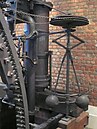
Centrifugal governor of a Boulton & Watt steam engine (1788)

Thermostat T86 of Honeywell , designed by Henry Dreyfuss (1953)
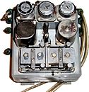
Pneumatic PID controller Telepneu from Siemens & Halske (approx. 1960)
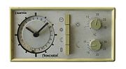
Time-controlled room temperature controller flexostat from Sauter (1967)

Hybrid anti-lock braking system from Bosch (1978)

Digital control unit for the active joint lock in the articulated bus from MAN (1986)

Compact controller RU 5X for heating systems from R + S controllers (approx. 2005)

Modular PLC ControlLogix of Allen-Bradley (2013)
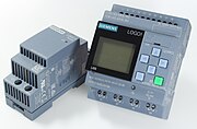
Compact PLC for small controllers Logo! from Siemens (2016)


.jpg)


Tools for rapid prototyping in research and development
In research and development, the problem regularly arises of testing new control concepts. The most important software tools for computer-aided analysis, design and rapid control prototyping as well as simulation of control systems are listed below.
- MATLAB and Simulink , The MathWorks
- Thanks to numerous toolboxes, a very extensive software package for numerical mathematics, suitable for simulation, system identification, controller design and rapid control prototyping (commercial)
- Scilab , Institut National de Recherche en Informatique et en Automatique (INRIA)
- Also very extensive software package for numerical mathematics with a similar concept and syntax as MATLAB, suitable for simulation, system identification and rapid control prototyping (free)
- CAMeL-View TestRig
- Development environment for modeling physical systems with a focus on controller design and rapid control prototyping as well as for connection to test stands (commercial)
- Maple
- Computer algebra system (CAS), masters numerical and symbolic mathematics, particularly suitable for some design methods of non-linear control (commercial)
- Mathematica , Wolfram Research, Inc.
- Comprehensive software package for numerical and symbolic mathematics (commercial)
- dSPACE
- Integrated hardware and software solutions for connecting MATLAB to test stands (commercial)
- LabVIEW , National Instruments (NI)
- Integrated hardware and software solutions for computer control of test stands (commercial)
- ExpertControl
- Software solutions for fully automatic system identification and fully automatic, model-based controller design for classic controller structures (PID controllers) as well as controller structures for higher-order systems (commercial)
- TPT
- Systematic test tool for control systems which, in addition to simulation, also offers results evaluation and analysis options.
All the tools listed show a high degree of flexibility with regard to the application and the controller structures that can be used.
Technical applications


- Railway technology
- A variety of control problems arise in drive control, for example torque and speed need to be controlled. Fuzzy control was successfully used on the Sendai subway .
- aviation
- Control problems occur in numerous components of aircraft, for example in the turbines, but also in relation to flight dynamics. Examples of flight dynamics control problems are the control of the roll, yaw and pitch angles, as well as the autopilot . See also flight controls .
- Energy Technology
- Position control of a control valve with an actuator within a controller cascade . In the interconnected power supply network, voltage and frequency must be maintained across the network. In every power plant, voltage and frequency are regulated locally, so that the task is solved with decentralized controllers by varying the control power (see also power plant management ). Globally, only the power setpoints of the individual power plants are specified.
- Automotive engineering
- Cruise control and anti-lock braking system (ABS), but also electronic stability program (ESP) are well-known controls in the vehicle sector, which are also referred to as driver assistance systems . Internal combustion engines also contain a variety of control loops, for example for idling speed, air ratio (see also lambda probe ), knock control (see also knocking (internal combustion engine) ). Modern automatic gearboxes require control loops for synchronization when shifting.
- Electric drive
- In vehicles with an electric drive, electric motors with greater powers are used. These are controlled via a speed and torque control, in hybrid vehicles also in connection with the combustion engine.
- pipeline
- In pipelines there are mainly meshed controls for flow , pressure control (inlet pressure, outlet pressure ) and position control including limit value control .
- robotics
- In production automation, the axes of the production robots must be positioned. A quick settling time and the slightest overshoot play a particularly important role here.
- process technology
- In process engineering, chemical and physical parameters are regulated that play a role in the process under consideration. Examples are the control of level, temperature, pH value and oxygen content of a stirred tank reactor or keeping substance or ion concentrations constant with a chemostat .
- Water management
- In order to avoid floods and secure the water supply, subordinate regulations of chains of dams are important. The filling level of an individual reservoir is specified by a higher-level management and regulated locally.
Tasks of the controller and associated design strategies
The controller's task is to approximate the controlled variable as closely as possible to the reference variable and to minimize the influence of disturbance variables. The reference variable can be designed as a fixed setpoint, as a program-controlled setpoint specification or as a continuous, time-dependent input signal with special follow-up properties for the controlled variable.
An excessively high loop gain that is not adapted to the controlled system can lead to oscillatory instability in controlled systems with several delay elements or even with dead time behavior. Due to the time delay in the controlled system, the control difference is fed to the controller with a delay via the set-actual value comparison. This lagging shift in the controlled variable can cause positive feedback instead of negative feedback at the setpoint / actual value comparison, and this makes the closed control loop unstable and builds up permanent oscillations.
Control loop design strategies for linear systems
The design strategies for control loops in linear systems relate to the optimization of the static behavior and the time behavior of the respective closed control loop. For example, the smaller the time delays in the controlled system, the higher the so-called loop gain and thus the gain of the controller can be selected, which improves the static accuracy of the control.
A high loop gain also makes the control loop dynamically fast, but it can only be implemented to a limited extent in practice because the manipulated variable cannot grow indefinitely due to technical stops or a lack of energy. A lower controller gain in connection with a temporally integral component of the controller makes the control loop for all static influences more precise and more stable, but also slower. To this end, an optimized compromise solution must be found using a suitable design strategy. To assess this, the term control quality was defined, which makes it possible to estimate the unavoidable periodically damped transient response of the controlled variable in control loops with higher-order controlled systems.
Control loop design strategy for mixed linear and nonlinear systems
The design strategy for mixed linear and nonlinear systems is more complicated and relates to models such as B. the Hammerstein model , in which a static non-linearity interacts with a dynamic linear system. The behavior of discontinuous non-linear static controllers in connection with linear controlled systems can be treated using the harmonic balance method.
Controllers in control loops with non-linear and linear components can be treated sensibly with numerical mathematics, especially with modern simulation tools such as those available for personal computers (PC).
Various theoretical and experimental analysis methods and mathematical design methods are used to determine the system behavior of the controlled system and the controller. The basics of mathematical treatment and the special procedures for control engineering follow in the following chapters.
As a simple, illustrative example of a standard control loop, room temperature control based on hot water central heating and its device components is intended to serve here.
Example of heating control in a building
Gas boilers, oil boilers and solid fuel boilers gain the thermal energy from the combustion of mostly fossil fuels and transport the thermal energy via the heat carrier water. A boiler heated by a combustion chamber is connected to a hot water circuit with radiators and / or underfloor heating with the help of a heating pump .
The heat supplied by the radiator heats the surrounding room air through convection and radiation. The thermal energy with the temperature gradient between the radiator and room temperature flows, depending on the size of the outside temperature, via the windows, doors, room walls and outside insulation to the outside weather.
Decentralized room temperature control
The amount of heat given off to the building is given by the difference between the flow and return temperatures on the boiler and the flow rate of the water. All radiators in the rooms of a building have the same flow temperature, which is usually controlled according to the outside temperature. The radiators in all rooms are equipped with thermostatic valves.
The size of the radiators is adapted to the respective room size. The flow temperature required for an existing outside temperature is recorded and controlled by an outside temperature sensor. Selectable heating characteristics from a characteristic field take into account the different heat requirements of buildings and thus the relationship between the outside temperature and the flow temperature. The aim is to automatically maintain the room temperature as a controlled variable at a desired setpoint with the help of a thermostatic valve .
With the thermostatic valve located on the radiator, the desired temperature of the room is set by turning the thermostatic cap within the range of a scale. The sensor of the thermostatic valve measures the current room temperature (theta) and changes the flow rate of the hot water through the radiator and thus the amount of heat supplied to the room via the valve position ( actuator ). The thermostatic valve has a proportional control behavior (P controller), which reacts somewhat slowly to disturbance variables when the deviation between the setpoint and actual value increases at low outside temperatures.

For the decentralized room temperature control as well as the central building temperature control with a reference living room, the use of a modulable burner with constant behavior of the heat energy generation applies to modern heating systems. This burner can, for example, continuously change its thermal energy in the range from approx. 10% to 100% depending on the requirements. The area of constant behavior of the burner is called the degree of modulation in terms of heating technology.
Condensing boilers with gas are able to extract and use almost all of the heat contained in the flue gases.
Compared to a heating system with intermittent on / off operation, the following advantages are associated with a modular burner:
- Low thermodynamic material stress in the burner chamber,
- Reduction of the burner noise and avoidance of expansion cracking noises in the pipelines,
- Fuel saving.
Below the inconsistent area of the burner, it works intermittently with a considerably reduced heat requirement.
Main controller for the reference living room
In addition to the decentralized temperature control of the living rooms with thermostatic valves, a reference living room (also pilot room, lead room, largest living room) is set up in modern heating systems, in which a central high-quality main controller via a room temperature setpoint generator and a reference room temperature sensor sets the flow temperature for the entire hot water circuit of the Centrally in the building and regulates the reference room temperature.
The temperature differences between the radiators and the cooler room air generate air movements ( convection ) and, to a lesser extent, radiant energy , which act on the sensor. The controller increases the flow temperature as required by switching on the burner or, if necessary, reduces it by switching off the burner.
For the quality of room temperature control, the structural room conditions and device arrangements such as radiators and the distance from the room temperature measurement location are also decisive. In an elongated room you cannot expect that a radiator with a thermostat at a distance of 10 cm will set a uniform room temperature over the entire room. On the other hand, a large distance between the radiator and the room temperature measurement location means that there is a longer signal delay ( dead time behavior ).
It is common practice to mount the sensor in the reference living room on the opposite wall of the radiator level. The sensor measures the air temperature, not the inner wall temperature. The radiators in the reference living room do not have thermostatic valves.
Designations for components and signals in the control loop
Annotation:
- In the German specialist literature, the control-related signal designations are not always taken from the valid DIN standards, but in some cases probably come from the representations of signal flow plans of dynamic systems in the state space. This theory, which originated in the USA by the mathematician and Stanford University professor Rudolf Kálmán , and the associated signal designations have remained unchanged since the 1960s.
- Some technical books on control engineering also show the designations X A (output variable) and X E (input variable) for the representation of signal inputs and signal outputs of transmission systems .

| designation | Signs as in state space systems | Symbol according to DIN IEC 60050-351 |
Meaning in general and in the example (room temperature control with thermostatic valve) |
|---|---|---|---|
| Controlled system | G S (s) |
|
|
| Disturbance | d | z |
|
| Controlled variable | y | x |
|
| actual value |
|
||
| Measuring element |
|
||
| Measurand | y M | y M |
|
| Reference variable | w | w |
|
| Setpoint |
|
||
| Control deviation |
e = w - y |
e = w - x |
|
| Regulator | G R (s) |
|
|
| Actuator |
|
||
| Control variable | u R | y R |
|
| Manipulated variable | u | y |
|
Definition of thermal energy
Colloquially, the thermal energy is somewhat imprecisely referred to as "heat" or "thermal energy". The thermal energy of a substance is defined as


where is the specific heat capacity , the mass and the absolute temperature . This definition assumes that the substance is within its physical state . For water, the liquid state applies in the temperature range from 0 (+) ° C to 100 (-) ° C at normal pressure at sea level .


A supply of heat increases the mean kinetic energy of the molecules and thus the thermal energy of a substance, a dissipation of heat reduces it.
If two thermal energy systems with different temperatures come together, their temperatures will equalize through heat exchange. This adjustment takes place until there is no longer a temperature difference between the systems. This process is known as heat transfer .
Without additional help ( energy ), thermal energy can never be transferred from the system of lower temperature to the system of higher temperature.
The heat flow or heat flow is a physical quantity for the quantitative description of heat transfer processes.
In physics and materials science, the interface or phase boundary is the area between two phases (here phase = spatial area of matter, composition and density of homogeneous matter). The interfaces between liquid and solid, liquid and liquid, solid and solid and solid and gaseous phases are called interfaces.
Alternative continuous and discontinuous regulation
There are two ways of regulating the reference room temperature as continuous or discontinuous regulation:
The change in the outside temperature is generally to be regarded as a static disturbance variable because the time response is very slow in relation to the change in the flow temperature. The heating controller can only react when the change in the outside temperature is noticeable through the external insulation and the mass of the building walls on the measuring sensor in the reference room.
The control of the room temperature in the reference room can usually be done conventionally using digital controllers that have to be adapted to the controlled system of the hot water circuit.
Industrially manufactured heating boilers are often designed with digital controllers using fuzzy logic . The basic idea of the fuzzy controller relates to the integration of expert knowledge with linguistic terms, through which the fuzzy controller is more or less optimally modeled using empirical methodology to a non-linear process with several input and output variables, without the mathematical model of the process (Controlled system) is present.
To put it simply, the application of fuzzy logic corresponds to the human way of thinking to recognize tendencies in the behavior of an unknown system, to anticipate and to counteract the unwanted behavior. This course of action is defined in the so-called “IF-THEN control rules” of a rule base.
Process of continuous and discontinuous regulation:
- The room temperature in the reference room can be regulated using a stepless controller that acts on a continuously operating mixing valve ( three-way mixer ) that accesses the boiler when there is a need for heat. This form of regulation is often used in apartment buildings.
- The room temperature of the reference room can be regulated using a two-point controller.
- This low-cost variant is particularly suitable for intermittent operation for cyclical switching on and off of the burner.
Discontinuous regulation
A discontinuous two-position controller without hysteresis has properties that correspond to a high loop gain . Whether it can be used to the full depends on the type of controlled system. This controller is particularly suitable for control systems that have to be controlled within wide limits for continuous power adjustment in intermittent operation (on / off operation).
The ratio of the maximum to the current heat energy requirement is given by the ratio of the switch-on / switch-off time:

The manipulated variable of the two-position controller determines the ratio of the switch-on time to the switch-off time, depending on the control deviation. The controller hysteresis and dead time behavior of the controlled system reduce the switching frequency. Special feedback from the two-position controller and the activation of a D component of the control deviation increase the switching frequency.
Calculation of the thermal energy flows
The behavior of the thermal energy flows can be calculated by using a block diagram with individual function blocks to show the dynamic time behavior of the thermal energy flows at the so-called interfaces (e.g. burner / boiler, radiator / air or interior / exterior walls / exterior weathering). The function blocks correspond to suitable mathematical models as system description functions.
Day and night reduction in room temperature
The storage behavior of the building walls and their insulation are of decisive importance for energy saving with the help of the so-called day-night lowering of the room temperature. With a constant low outside temperature and a longer-term room temperature reduction, the energy-saving potential is great. If the room temperature drops briefly, the building walls then have to be heated up again without the boundary surfaces in the masonry and the insulation becoming stationary, which would make it possible to save energy.
Externally controlled flow temperature limitation
The heat requirement in living spaces is several times higher in the very cold winter than in the transition period between autumn and spring. For this reason, the flow temperature of the heating circuit is limited by means of a precontrol via a controller depending on the outside temperature, so that large overshoots of the room temperature (controlled variable) as well as heat losses are avoided.
The radiator temperature is usually not measured, it is recorded from the mean value of the flow temperature and the return temperature at the boiler. Heat losses from the insulated pipelines are neglected.
The characteristic curve for limiting the flow temperature of the heating circuit as a function of the outside temperature can be set in commercial systems and is dependent on the climate zone . The limited flow temperature must be slightly higher than the value that is required for the heat demand of the set reference room temperature setpoint. The limitation control of the flow temperature as a function of the outside temperature can be carried out using a simple two-point controller.
Disturbance variables of the heating control circuit
Disturbance variables in room temperature control are changes in the generation of heat energy through intermittent operation. B. the effects of fluctuations in gas pressure (gas boiler) or changes in the calorific value of the heating oil (oil boiler) are negligible.
The main short-term disturbances affecting room temperature are open doors or windows and solar radiation in the window area.
The main disturbance factor in building heating is the influence of the outside temperature. The change in outside temperature and the influence of wind and precipitation are long-term disturbances due to the heat storage capacity of the building mass.
Disturbance variables can attack all part of the controlled systems. Short-term disturbance variables have a slight influence on the actual value of the controlled variable if they occur at the input of the controlled system. Disturbance variables on controlled systems have the greatest influence when they occur at the output of the controlled system.
The assessment of a linear control loop with a reference variable jump is calculated using the reference variable transfer function.
The assessment of the disturbance behavior of a linear control loop on a linear controlled system is often calculated using a disturbance jump with the disturbance variable transfer function.
Stationary or abrupt or pulse-like disturbance variables in the control loop can be taken into account positively or negatively in a graphical signal flow diagram using an addition point.
The most dominant disturbance variable in the control system of a heating system, which changes within wide limits, is the heat energy outflow from room temperature via the building walls to the outside weather. While the influence of a disturbance variable on any control loop only shows technical information or a required specific behavior of the controlled variable, the disturbance variable of the energy flow of a building temperature control to the outside weather means an energy cost factor of considerable extent.
The energy flow to the outside weather is under normal operating conditions, i. H. closed windows and doors, depending on:
- from the outside weather, such as outside temperature, sun, wind and rain,
- the quality of the building's thermal insulation .
- The better the outside insulation, the lower the radiator temperature can be for a given outside temperature.
- on the size of the reference room temperature
- Every reduced degree Celsius of an individual “feel-good room temperature” reduces the radiator temperature considerably in percentage terms.
- from the size of the dominant time constants of the three mathematical sub-models of the radiator temperature to the room temperature to the outside temperature.
- For constant outdoor weather conditions and a given target value for the reference room temperature, after a sufficiently long time, an equilibrium condition is established between the heat energy generated and the heat energy flowing off through the building.
Simulation of a heating control circuit with partial models

Task: Calculation of the temporal behavior of the mean radiator temperature and the room temperature of a reference living room for the room temperature setpoint specification from 5 ° C to 20 ° C at a stationary outside temperature of −10 ° C. Wind and precipitation should not change for this process.
The signal flow diagram of the simulation of the reference room heating control shows the relationships between the sub-models.
Data specification for the heating control circuit For a rough calculation of the control process for the room temperature in the reference room, simplifications and numerical assumptions must be made from experience. The following data are given:
- maximum flow temperature: 80 ° C
- Room temperature setpoint: 20 ° C
- stationary outside temperature: −10 ° C
- Outflow of heat energy (in ° C) is measured empirically:
- For a mean stationary radiator temperature of 60 ° C and a stationary outside temperature of −10 ° C, a room temperature of 20 ° C is reached after a sufficiently long time.
- With this information, a room temperature change of 1 ° C corresponds to the ratio of the differential values of the radiator temperature to the room temperature with reference to the outside temperature:
- Factor = [60 ° C - (−10 ° C)] / [20 ° C - (−10 ° C)] = 2.33 ° C per 1 ° C change in room temperature
- Limited mean radiator temperature at −10 ° C outside temperature: 70 ° C
- Selected stationary initial value of the room temperature in frost protection mode as setpoint: 5 ° C
- Calculated stationary initial value of the mean radiator body temperature in frost protection mode:
- For a required stationary reference room temperature of z. B. 5 ° C, d. H. Room temperature reduction of 15 ° C results in a required radiator temperature of:
- Radiator temperature = 60 ° C - 2.33 15 ° C = 25 ° C.
Definition of the partial models based on the estimated data specification
For the dynamic process of the setpoint changes with reference to the radiator temperature, the room temperature and the heat energy outflow, the initial conditions of the individual systems must be taken into account.
- Partial model 1: Heat energy generation from the burner to the radiator temperature
- The heat energy generated in the burner and boiler is pumped through all pipes and radiators as the flow temperature with the heating pump and appears again on the boiler as the return temperature. The mean radiator temperature is taken as the mean value of the flow and return temperatures.
- Data:
- Tt = 4 [minutes], T E = 60 [minutes] with an increase, T E = 100 [minutes] with a decrease in heating energy:

- Partial model 2: radiator temperature to room temperature
- The heat energy given off by the radiators heats the room air, which rises first on the windows and then up to the ceiling and cools down. This leads to air turbulence via convection and radiation , which reaches the room temperature sensor even after a dead time and settling time.
- The measured and controlled reference room temperature is not identical to the inside wall temperature, the floor and ceiling of the reference room, through which the thermal energy flows away to the outside weather (as a representative for all rooms).
- Data:
- Tt = 10 [minutes], T E = 200 [minutes] with an increase, T E = 300 [minutes] with a decrease in heating energy:

- Partial model 3: room temperature to the inside of the building wall to the outside to the outside
- The mathematical model for the dissipation of heat energy from the room air via the windows and the building walls to the exterior insulation and the exterior weathering is very complicated and is therefore simplified.
- The partial model 3 consists of a static part, which shows the relationship between radiator, room and outside temperature using a straight line equation, and a dynamic part, which takes into account the storage capacity of the building walls and insulation.
- Depending on the nature of the mass of the room walls (heat storage capacity, thermal conductivity, internal thermal insulation, proportion of internal and external walls) and the insulation material on the outside, it can be a complicated system of a higher order with a large dominant time constant. To simplify this sub-model 3, a first-order delay element (PT1 element) with a large equivalent time constant is selected as the dynamic system behavior.
- For the simulation of the energy flow, there is a static relationship with this information that can be determined by a straight line equation.
- Simplified model of the time behavior:

- Assuming a linear relationship between the radiator temperature and the selected room temperature at constant outside temperature, the value of the radiator temperature can be calculated from straight line equations for various room temperature values.
- General straight line equation with X as input variable and Y as output variable:

- Static relationship of partial model 3
- A straight line equation is used to determine which value must be subtracted from the filtered radiator temperature (= output model 2) as a function of the outside temperature so that the room temperature results as a control variable.
- For a room temperature of 20 ° C, the associated radiator temperature is given as 60 ° C. For another value of the room temperature, the associated radiator temperature can be calculated from the proportion of the temperature differences to −10 ° C:

- For static model 3, the difference [radiator temperature - room temperature] is required. This value is subtracted from the output of model 2:
![[\ theta _ {\ text {Radiator temperature - room temperature}}] = 13 {,} 33 \ + \ {\ frac {40-13 {,} 33} {20}} \ \ cdot \ [\ theta _ {\ text {Room temperature}}]](https://wikimedia.org/api/rest_v1/media/math/render/svg/9b7e1dde8ff3c2acc2ea428c2d0ae5e1a0b2d8f4)
- This results in the static values for the setpoint jumps in the room temperature, the associated values for the radiator temperature and all intermediate values:
-
- Setpoint room temperature 20 ° C:
- [Radiator temperature] - [Radiator temperature - room temperature] = [room temperature] = 60–40 = 20 ° C
-
- Setpoint room temperature 5 ° C:
- [Radiator temperature] - [radiator temperature - room temperature] = [room temperature] = 25–20 = 5 ° C
Graphical representation of the temperature values of the heating control

Task Based on the partial models of the controlled system, the graphical course of the radiator temperature and the room temperature from the frost protection mode to the operating status should be calculated and graphically displayed.
- Commercial computer programs are ideal for calculating transmission systems or simulating control loops. With the most popular programs such as MATLAB and Simulink, extensive instruction sets are available for the theoretical modeling of dynamic systems and many special control commands.
- Alternatively, linear systems can be calculated numerically with the help of difference equations. Non-linear systems such as the two-position controller can be easily calculated with the help of IF-THEN-ELSE instructions. A calculation sequence refers to a chain of systems connected in series, starting with the input signal and ending with the output signal. Each sequence k relates to the discrete time k · Δt.
For a better understanding, two diagrams with the static and dynamic behavior of partial model 3 are shown.
- Graphic representation of the temporal behavior of the temperature values without heat storage of the building walls (partial model 3 with T = 0).
- Graphic representation of the temporal behavior of the temperature values with heat storage of the building walls (partial model 3 with T = 500 [minutes]).
Critical assessment of the simulation results
- In principle, the calculated time curves for the radiator temperature and the room temperature correspond to realistic heating controls.
- Reliability of the mathematical models
- The simulation of a dynamic process is as good as the quality of the mathematical models of the controlled system.
- Model 1 (heat energy generation to the radiator) can largely correspond to reality.
- Model 2 (heating of the room temperature) is physically connected to model 1, but cannot guarantee that model 1 is free of interference due to the larger time constants. It acts more than a 1st order low-pass filter on the sawtooth change in radiator temperature.
- Model 3 (outflow of thermal energy to the outside weather) subtracts from the output value of model 2 the portion of the outwardly flowing thermal energy. Although Model 3 is a system with distributed energy storage, it is treated as a system with a concentrated energy storage for reasons of easier predictability. This results in the controlled variable room temperature as a function of the radiator temperature and the outside temperature.
- The time constants of all sub-models are estimated.
Graphic representations of the temperature values

For a better understanding, the control processes are shown in 2 diagrams, statically without the stored thermal energy of the walls and dynamically with the stored energy of the walls. This is the third partial model, the time constant of which is set once to a value for T = 0 and T = 500.
The following shows the simulation of the model of the building heating control loop for a jump in the setpoint from frost protection mode 5 ° C to operating mode 20 ° C.
Comment on the illustration of the simulation with the third partial model without storage capacity of the room walls The calculation of the flow of thermal energy from the initial values to the final values is carried out purely statically without stored thermal energy in the building walls.
The setpoint jump takes place after 200 minutes. The simplified static partial model 3 as a PT1 element with the behavior of the time constant T = 0 shows the steady-state conditions of the radiator temperature and the room temperature, which are established after a sufficiently long time. The transition from the lower temperature values to the upper temperature values is not real in time because the stored heat of the building walls is not taken into account for each value of the radiator temperature and the room temperature.
Comment on the illustration of the simulation with the third partial model with storage capacity of the room walls The calculation of the flow of thermal energy from the initial values to the final values takes into account the stored thermal energy of the building walls.
The setpoint jump takes place after 200 minutes. The simplified static partial model 3 as a PT1 element for the heat storage capacity of the room walls with the time constant T = 500 minutes shows the behavior of the rise in radiator temperature and room temperature. It becomes clear that the room temperature has already reached the target value of 20 ° C, while the radiator temperature is only required at 45 ° C due to the stored thermal energy of the walls. Only after approx. 2000 minutes does the radiator temperature of 60 ° C become static, assuming constant weather conditions.
Mathematical methods for describing and calculating a control loop
This chapter shows the application of the methods of control engineering and system theory for the calculation of dynamic systems and control loops. The terms of methods of system descriptions, transfer functions, linear and non-linear controlled systems, time-invariant and time-variant systems, two-point controllers, mathematical system models and numerical calculations are touched upon and help is given in detailed articles or their chapters.
A dynamic system is a functional unit with a specific time behavior and has at least one signal input and one signal output. Models ( modeling ) of a real dynamic transmission system are mathematically described by:
- Differential equations
- Transfer function and frequency response
- State space representation
- Numerical time-discrete description of linear systems ( difference equations ) and non-linear systems (logical commands, table values)
Ordinary differential equations
A differential equation (DGL for short) is an equation that contains one or more derivatives of an unknown function. Different physical problems can be represented formally identically with DGL-en.
If derivations only occur with respect to one variable, one speaks of an "ordinary differential equation", whereby the term "ordinary" means that the function under consideration only depends on one variable. Many dynamic systems from technology, nature and society can be described with ordinary DGL-s.
A linear DGL contains the function you are looking for and its derivatives only in the first power. There are no products of the function sought and its derivatives; Likewise, the function you are looking for does not appear in arguments of trigonometric functions, logarithms, etc.
Creation of a differential equation A differential equation is a determining equation for an unknown function. The solution to a DGL is not a number, but a function!

Example of an electrical oscillating circuit: Voltage balance: According to Kirchhoff's 2nd theorem, the sum of all voltages in a mesh is zero.

The voltage drop across the resistor R results from U R = i · R. According to the law of induction, the voltage across the inductance U L = L · di / dt. The charging current across the capacitor is proportional to the voltage change across the capacitor i (t) = C · dy / dt.
The application of the mesh theorem leads to a first order differential equation:

If we put in the DGL for i (t):

one, then the oscillation equation results:

Time constants such as T 1 = R * C and T 2 ² = L * C can be introduced. If you also replace the representation of the input variable and output variable that is usual in the system description , then the well-known DGL for a series resonant circuit is:

Basics of the transfer function as a system description

The most frequently presented system description of linear time-invariant systems is the transfer function with the complex frequency . It is successfully used for system analysis, system synthesis, system stability and allows the algebraic treatment of arbitrarily switched, reaction-free subsystems.


A transfer function describes the dependence of the output signal of a linear , time-invariant system ( LZI system ) on its input signal in the image area (frequency area, s-area). It is defined as the quotient of the Laplace transformed output variable to the transformed input variable :


The Laplace transformation is an integral transformation which can be used to transfer a time function into an image function with the complex frequency . The image function can again be represented as a time function using various mathematical methods.


Dynamic time-invariant systems with concentrated energy stores (e.g. spring-mass-damper systems or electrical L, C and R elements) are described by ordinary differential equations with constant coefficients. When the system is idle, the energy stores have the value zero.
To simplify the calculation and to make it easier to understand, the differential equation is subjected to a Laplace transform . According to the Laplace differentiation theorem, a 1st order derivative of the differential equation is replaced by the Laplace variable s as a complex frequency. Higher derivatives of the nth order are replaced by .

Example of an ordinary differential equation with constant coefficients:

The Laplace transform of the differential equation is:

The coefficients a and b of the differential equation are identical to those of the transfer function.
The result of the transformation is defined according to the order of the terms of the resulting polynomial as the ratio of the output variable to the input variable as a transfer function. The transfer function G (s) can always be written as a fractional-rational function . Since the transfer function is used to describe the input-output behavior , the transfer system should have an output variable equal to zero for a given input variable at a given point in time .


Factoring the transfer function in the s domain
By determining the zeros , the polynomials of the transfer function can be brought into a product form ( linear factors ) in the numerator and denominator. The poles (zeros of the denominator) or zeros (zeros of the numerator) are either zero, real or conjugate complex . The product representation in the numerator and denominator of the transfer function is mathematically identical to the polynomial representation.


The poles and zeros of the transfer function are the most important parameters of the system behavior.
Example of a transfer function of the polynomial representation and the decomposition into the pole-zero representation with real linear factors:

Linear factors:
- In the case of linear factors of the first order, the zeros or poles are real numerical values. Stable systems contain negative real parts.
- Second degree linear factors with complex conjugate zeros or poles are combined into quadratic terms for easier calculation, in which only real coefficients occur.
- Linear factors are mostly converted into the time constant representation by the reciprocal formation of the zeros and poles.
- Product term in the time constant representation with a negative value of the zero :

In linear control technology, it is a welcome fact that practically all regular (phase-minimal) transfer functions or frequency responses of control loop elements can be written or traced back to the following three basic forms ( linear factors ). They have a completely different meaning, depending on whether they are in the numerator (differentiating behavior) or in the denominator (delaying, integrating) of a transfer function.
Depending on the numerical values of the coefficients and the polynomial representation, the products can take the following three forms in the time constant representation:


Type linear factor Meaning in the counter Meaning in the denominator
(Zero position = 0)Differentiator, D-member Integrator, I-link
(Real zero)PD link Delay, PT1 element
(Zeros conjugate complex)PD2 element: for 0 < D <1 Vibration link PT2 link : for 0 < D <1


- Here, T is the time constant, s is the complex frequency, D degree of damping.
The transfer function of a dynamic transfer system can contain single and multiple linear factors in the numerator and denominator.

Definition of the variables s
- is the independent variable in the complex frequency domain (image area, s-area) with as real part and as imaginary part. It allows any algebraic operations in the s-domain, but is only a symbol for a completed Laplace transformation and does not contain a numerical value. Exponents of correspond to the degree of the derivative of the differentials .
- Numerical values are created from the coefficients and the polynomial representation in that the polynomials of the transfer function are broken down into linear factors (products) by decomposing zeros. These zeros or poles can be zero, real or complex conjugate.
- The real parts and the imaginary parts of the zeros or poles can, depending on the numerical values of the coefficients, and also have the numerical value zero. This creates the three forms of linear factors z. B. in the denominator of the transfer function with the behavior integration, delay, delay 2nd order conjugate complex.


Table of all occurring types of regular transfer functions in time constant representation:
Name → P element I-link D link PD 1 link PT 1 link PT 2 link (oscillating link ) PD 2 link Dead time element Transfer function G (s) Poles and zeros no no Transition function
(step response)


graphically not representable 


Notes on the transfer function
- The great advantage of describing linear dynamic systems as transfer functions with the linear factors is that there are only six easy-to-remember basic forms of system behavior that can be combined to form larger system forms. The transcendent form of the non-linear dead time element does not belong to it, unless it is approximated to the behavior of the dead time element as a fractional rational function .
- In connection with other system descriptions such as the differential equation, difference equation, state space representation and mixed linear and nonlinear models, naming transfer systems as transfer functions is advantageous because the system function is so well known.
- The transfer functions can be combined as individual transfer systems in the series and parallel connection of a block diagram and treated algebraically.
- The gains of the -Gliedes and -Gliedes can also be written as time constants .
- The transfer functions shown with components are called "ideal". These systems cannot "real" be produced without a combination with a delay element ( element). The time constant of the delay element must be significantly smaller than that of the D component.


- Example of a real -link with T V ≫ T:
- The numerical calculation of ideal components works with the help of the difference equations without any problems. No infinitely large edges can arise during the differentiation, because calculations are made over time .
- Conclusion: In the numerical calculation, an ideal -link fully compensates for a -link with the same time constants to the factor .


- The differentiating form of the 2nd order transfer function ( -member) with conjugate complex zeros allows the compensation of the delay element 2nd order with conjugate complex poles with the same time constants and the same degree of damping.

- Application: Pre-filter in the control loop input reduces damped oscillations of the controlled variable and thus allows a higher loop gain.
- The transfer functions are always written as fractional-rational functions.
- The transcendent function of the dead time element can be multiplicatively attached to the transfer function of a system . This form of the transfer function as a complete system is only suitable for frequency response analyzes. Any algebraic operations with a dead time element are not permitted.
- Non-regular transfer functions contain a minus sign in the equation (= positive zero). They can arise through positive feedback (= positive feedback) and behave monotonically unstable. With any input excitation , the output variable of an unstable element strives for an infinitely large value up to its natural limit, depending on the time constant .


Example of the notation of a first-order delay element with the gain factor :

These kinds of equations of the transfer functions can be treated algebraically, apply to linear systems and relate to time-invariant behavior. Transfer functions can be combined algebraically with any linear factors to form controlled systems and control loops, as long as no dead time system is included. If an input signal is given as a test signal , the time behavior of the output signal can be calculated using Laplace transformation tables .
Transfer functions as a block structure in the signal flow diagram
Transmission systems can be grouped as blocks from subsystems. The superposition principle applies . The systems in the product display can be moved in any order. The system outputs must not be loaded by subsequent system inputs (freedom from feedback).
- Parallel connection:

- Equation of the transfer function of the parallel connection:

- Series connection:

- Equation of the transfer function of the series connection:

- Negative coupling or feedback:

- Equation of the transfer function of the negative feedback:

- In the case of a control loop that does not contain a static or dynamic subsystem in the negative feedback branch, the system G 2 (s) = 1.
-

- The transfer function of the closed control loop is thus:


- A positive feedback is a positive additive acting return of the signal output to the system input. Depending on the magnitude of the gain of G 1 (s), it leads to monotonous instability or a hysteresis effect.
- Equation of the transfer function of the positive feedback:

- With G 1 (s) as an open control loop, any algebraic combinations of the subsystems of the controller and the controlled system are understood.
Linear controlled systems
Linear systems are characterized in that the so-called superposition law and the reinforcement law apply. The superposition theorem states that if the system is excited with the time functions f1 (t) and f2 (t) at the same time, the system response is also formed from a superposition of the system response of f1 (t) and the system response of f2 (t).
The amplification principle means that with double the amplitude of the input function, the system response is also twice as large.
Natural linear controlled systems often contain delaying, integrating and dead time subsystems.
An electrical resistance capacitor low-pass filter of the 1st order in the reaction-free state with the time constant T = R C is described by the following transfer function:
1st order delay element (PT1 element):

To calculate the time behavior of transmission systems G (s) with the transfer function, the input signals (test signals) must be defined in the s range.
For the calculation of the step response of a system in the time domain, the standardized step 1 (t) as a Laplace-transformed test input signal is U (s) = 1 / s.
The equation for calculating the time behavior of the PT1 element can be read directly from the Laplace transformation tables:
Searched function in the s-area:

Associated function in the time domain:

The factor K is not subject to the transformation and is therefore valid in the s domain as well as in the time domain.
If the corresponding time function of a transfer function is searched for in time constants or zeros representation in the transformation tables without the Laplace-transformed input signal, the result is always the impulse response of the system.
Linear types of controlled systems
The time constant T means for a first-order delay element that an output signal has reached approx. 63% of the value of the input signal after a jump in an input signal and the signal curve asymptotically - after approx. 3 to 4 time constants - approaches the maximum value of the input signal.
- A first-order delay element ( PT1 element ) behaves invariably when the time behavior ( time constant ) does not change for a rising (jump) or falling (return) input signal u (t) . This is explained by the associated ordinary differential equation with constant coefficients.
- A 2nd order delay element with complex conjugate poles, e.g. B. a damped spring-mass system is referred to as a vibrating member. Depending on the degree of damping D, the step response approaches the maximum value of the input variable as the oscillation fades away.
- A controlled system with several PT1 elements is called a controlled system with compensation, also known as a global ( proportional ) P behavior.
- A controlled system with several PT1 elements and an I element is called a controlled system with global I behavior.
- A controlled system with dead time with delay elements cannot be calculated arbitrarily algebraically. Unless the dead time is roughly defined as a fractional-rational function with delay elements.
Advantage of the system description with transfer functions (without dead time behavior)
- Simple algebraic calculation of any system links of all individual systems possible
- Control loop elements of the controller and the controlled system of the open loop can be closed to form a control loop. The resulting polynomials can be broken down into poles and zeros and again written as factorial basic elements (linear factors), mostly in time constant representation.
- All system properties can be read from the pole zero representation.
- With the graphic methods “locus of the frequency response” and the “stability criterion from Nyquist”, the stability of the closed control loop can be determined on the basis of the individual systems G (s) of the open (cut) control loop.
- For a known Laplace-transformed test input signal such as the step function or shock function, the time behavior of an individual system or a control loop can be calculated and graphically displayed using Laplace transformation tables.
- Regulator design
- Controlled systems can be simplified if delay elements (PT1 elements) are compensated by PD1 elements of the controller.
Transfer function and frequency response
The transfer function is a non-measurable function of the ratio of the Laplace-transformed output variable to the input variable. It can be converted into the frequency response with identical coefficients (time constants) at any time .
The frequency response is a special case of the transfer function.

In contrast to the transfer function, the frequency response of a linear transfer system can be measured by exciting the unknown system with a sinusoidal input signal of constant amplitude with variable frequency and recording the output variable. The genesis of the frequency response and the transfer function are different, the spellings can remain identical.
With the graphic methods "locus of the frequency response" and the "stability criterion from Nyquist", the dead time behavior of a subsystem can also be treated, because these methods relate to the open control loop.


Time-invariant and time-variant controlled system components
Example building heating: In a heated building, the heat generated flows from the radiator via the room air to the building walls via the insulation to the outside weather. The different heat flows between the masses and the associated insulation each have a specific time behavior that must be defined for an analysis of the entire controlled system.
Time invariance
The dynamic systems presented so far are time-invariant systems with concentrated energy stores.
A dynamic transmission system is time invariant if it does not change over time, i.e. that is, the system response to an identical input signal is independent of. The coefficients of the mathematical system description are constant (unchangeable over time, invariant).


A time-invariant delay element (PT1 element) behaves identically for a signal input jump as well as for a signal return jump, i. In other words, it always asymptotically strives for the maximum value when jumping or the starting value with the same time constant when jumping back.
Time variance
For the description of a dynamic system e.g. B. a heat flow in a homogeneous material (water, air, stone) is a system with spatially distributed energy storage.
A time-variant system behaves differently at different times. In technical systems, the reason for this is mostly in time-dependent parameter values, for example by changing the coefficients of the energy stores [time-dependent coefficients of the derivatives ].
In many processes, the effects of time variance are so small or slow that these systems can be treated approximately as time-invariant.
The ordinary differential equations associated with the transfer functions have constant coefficients. Constant coefficients mean that the time behavior of the system does not change. Is z. If, for example, the time behavior of an accelerated mass is described and it is an accelerated rocket that changes its mass, then it is a time-variant process.

Mathematical time-variant model of the heat flow in a homogeneous medium e.g. B. Air
The transfer behavior of a signal jump in a spatially homogeneous medium (material) is shown in its time behavior between two measuring points approximately as a first-order delay element with a dead time and different time constants.
After recording the step response, the mathematical model for the heat flow in a homogeneous medium can be approximated by a simple model with a PT1 element and a dead time element. The parameters of the equivalent dead time and the equivalent time constants can be determined experimentally on the basis of a measurement protocol to be recorded.


For building heating, it is taken into account that the boiler heats up quickly and cools down slowly due to the thermal insulation. The same applies to the flow of energy from the radiator to the room air and via the walls to the outside weather. Such systems behave in a time-variant manner , i. In other words, the system has a different time constant for a signal jump than for a signal jump back. The better the insulation of a heated medium, the more different the time constants for heating (small) and heat flow (large).
If the representation of the dead time with the computer program causes problems, the model equation shown can also be practically identical by a very good approximation with equivalent dead times by z. B. n = 3 PT1 elements can be represented as follows:

Non-linear transmission system
The linear system property is often not given, since many interacting systems such. B. in control engineering for valve characteristics, manipulated variable limits or switching processes do not have linearity.

A nonlinear system can appear either in the form of nonlinear static characteristics or in the form of nonlinear operations such as multiplication or division of variables in algebraic equations and differential equations.
A non-linear dynamic system of the 2nd order arises, for example, from a spring-mass-damper system if the spring system or the damper has a non-linear behavior. Given the multitude of forms of nonlinear systems, it is difficult to classify them into specific classes. Nonlinear systems can be classified as unique.
In the case of non-linear transmission systems, at least one non-linear function acts in conjunction with linear systems. These non-linear functions are differentiated according to continuous and discontinuous non-linearities. Continuous non-linearities do not show any jumps in the transfer characteristic, such as B. with quadratic behavior. Discontinuous transfer characteristics such as limitations, hysteresis, response sensitivity, two-point and multi-point character do not have a continuous course.
The principle of superposition does not apply to non-linear transmission systems.
The following relationships arise with non-linear systems:
- If a non-linear transmission system is operated at a fixed operating point, the non-linear behavior of the system can be replaced by a linear model for the immediate vicinity of the operating point.
- Every non-linear relationship can be described approximately linearly in the small-signal behavior. The approximation becomes better, the smaller the difference quotient is at the operating point.
- If a non-linear function is given as a graphical characteristic curve, the slope of the tangent for the linearized relationship can be determined by creating a tangent at the desired operating point
- A non-linear dynamic system with a continuously falling or rising characteristic can also be linearized by incorporating it into its own control loop and thus its dynamic behavior can also be improved.
- Nonlinear differential equations can usually only be solved numerically. If a transmission system can be broken down into subsystems and the nonlinear behavior of individual systems is available as an analytical equation or table of values, the behavior of a nonlinear dynamic system can be calculated relatively easily.
- The interaction of discontinuous, non-linear, static systems with linear systems to form control loops can be optimized with the graphic method of harmonic balance . The application of harmonic balance for the analysis of non-linear control loops with the clear two-locus method shows when permanent oscillations occur and how permanent oscillations can be avoided.
- Flatness Based Systems
- Flatness in systems theory is a system property that extends the notion of controllability of linear systems to nonlinear systems . A system which has the flatness property is called a flat system.
- The flatness property is useful for the analysis and synthesis of nonlinear dynamical systems. It is particularly advantageous for trajectory planning and asymptotic follow-up control of non-linear systems.
Basics of the numerical calculation of dynamic transmission systems
Relatively simple transmission system structures with non-linear elements can no longer be solved in a closed manner by conventional calculation methods in the continuous time domain. With commercially available personal computers, the behavior of any meshed system structures can be determined relatively easily by means of numerical calculation.
For the implementation of the calculation of transmission systems or the simulation of control loops, commercial computer programs are available. With the well-known programs such as MATLAB and Simulink , extensive instruction sets are available for the theoretical modeling of dynamic systems and many special control commands.
Alternatively, you can use your own computer programs to perform very efficient control loop simulations using difference equations in conjunction with logical operators. Relatively little mathematical knowledge is required.
If limitation effects occur in the controller or dead time systems in the controlled system, or the controller has non-linear properties like the two-point controller, the time behavior of the control loop can only be calculated numerically with the discrete time . The calculation of dynamic systems with the method of the state space representation is also not possible with a dead time system without numerical calculation.
The numerical calculation allows a complete overview of the inner movement of dynamic transmission systems in tabular and graphical form. In connection with logical program commands and value tables, non-linear, limiting and dead time systems can be simulated.
Method of numerical calculation
If the differentials of the output variable y (t) of a differential equation are replaced by small difference quotients with a discretized time, a numerically solvable difference equation is created that approximates the differential equation. It is useful to convert linear elementary systems (transfer functions such as I, PT1, D, PD1 elements) into difference equations. Depending on the position of the function blocks in the signal flow diagram, these can be treated recursively with non-linear systems or systems with dead time and their numerical calculation methods.

Difference equations or a chain of difference equations that describe several elementary systems connected in series allow the output variable to be calculated algebraically for a small time step depending on the input signal . The numerical overall solution of the system takes place - with simple difference equations - recursively over many calculation sequences in small constant time intervals. The form of the overall solution is thus in tabular form. All rows contain the same difference equations of the calculation sequence, all columns calculate the sequence . The line with is reserved for initial values. The total time period considered for the numerical solution is . The output variable follows each calculation sequence in amplitude steps at a time interval .


Difference equations of linear systems
With the help of the system descriptions as transfer functions G (s), the number of the few different elementary systems (linear factors in the numerator and denominator of the transfer function) is determined. The difference equations derived therefrom exist from the associated system-describing differential equations.
The simplest difference equations are created using the " Euler's route train method " (also known as the rectangular method ). Other methods are used for a better approximation e.g. B. instead of the rectangle method ( explicit Euler method ), the trapezoidal surface method ( Heun method ), the multi-step method ( Runge-Kutta method ) and other methods.
With the following list of the difference equations of the transfer elements G (s) of the first order, all linear systems of higher order - including systems with conjugate complex poles - can be simulated. Difference equations can be used with any programming language. The use of the spreadsheet is recommended because it eliminates program errors.
Associated difference equations of first order transmission systems G (s):
| Elementary systems | Transfer function | Difference equations |
|---|---|---|
| P element | ||
| I-link | ||
| D link | ||
| PD 1 link | ||
| PT 1 link |


![{\ displaystyle y _ {(k)} = [u _ {(k)} - u _ {(k-1)}] \ cdot {\ frac {T} {\ Delta t}}}](https://wikimedia.org/api/rest_v1/media/math/render/svg/ce6e53f3d979ff1b6f2b440cfe0b46ac00c14c2e)

![{\ displaystyle y _ {(k)} = K_ {PD1} \ cdot \ left [u _ {(k)} + (u _ {(k)} - u _ {(k-1)}) \ cdot {\ frac {T } {\ Delta t}} \ right]}](https://wikimedia.org/api/rest_v1/media/math/render/svg/c8fa2c69014ea947d0255bba0bfb99e9a2ebc884)

![{\ displaystyle y _ {(k)} = y _ {(k-1)} + [K_ {PT1} \ cdot u _ {(k)} - y _ {(k-1)}] \ cdot {\ frac {\ Delta t} {T + \ Delta t}}}](https://wikimedia.org/api/rest_v1/media/math/render/svg/23d0fda8865ca44b3e33ceb29573b186d1949667)
(With = gain factor, = current discrete-time output variable, = previous output variable, = time constant, = current discrete-time input variable)

Nonlinear Static Systems
The tabular form of the numerical solution also allows the calculation of non-linear static systems by assigning the non-linear relationship as a table of values to the table column of the calculation sequence. It is also possible to calculate the dead time of a system by shifting the lines with suitable program commands. In non-linear systems such as the discontinuous static multi-point controller, the numerical description consists of simple non-linear equations. The logical description can be made with the IF-THEN-ELSE statement. Non-linear, discontinuous static characteristics that cannot be described using analytical equations can be inserted as value tables within the overall table. The numerical calculation of non-linear functions can also be used for static systems without time behavior, if z. B. the interval is related to the system input variable.


Application of numerical calculation

- Simulation of dynamic systems
- In the case of a control system for recognizing the control properties, the behavior of the controlled variable due to a sudden change in the setpoint is often of interest. The behavior of the controlled variable in the event of a sudden or constant change in a disturbance variable is also of interest. Usual system tests of any physical controlled variables of control loops relate to an input signal z. B. with a setpoint change for a certain point in time to a sudden, standardized input signal from zero or from the rest position to 1 = 100%. The behavior of the step response is analyzed to determine whether it is within the desired limits.
- With the simulation of a mathematical model of a transmission system or a control loop, it is possible to carry out a system analysis or a system optimization with suitable test signals.
The advantage of simulating on a model is obvious. No technical systems are endangered or required. The time factor does not matter, very fast or very slow processes can be optimized. The prerequisite is the mathematical description of a well-approximated model of the mostly technical controlled system.
For the numerical calculation of the time behavior of control systems with dead time, there are no other alternative methods with regard to the analysis and optimization of systems when using commercial programs or simple programs with difference equations.
- Digital regulation online
- In real-time calculations, for example with a programmable digital controller that acts on a hardware control system, the discretization time is (often ) replaced by the "sampling time" with which the mostly analog input and output signals of the control system are recorded via analog-digital converters. The sampling of the input and output signals is usually followed by a holding element (sample-and-hold method), so that the input and output signals are graded. In the case of fast controlled systems, the system speeds of the computer, the A / D converter, the sample-and-hold circuit, as well as the difference equations used or their approximation algorithms play a major role.

- Initial values of the internal energy storage of a dynamic system
- Initial values of a dynamic system mean that the internal system memories do not have the value zero at time t 0 . With difference equations of dynamic systems, the initial value of the output variable y (t) or y (k · Δt) can also be calculated by giving all delays the same initial value.
For the calculation of the initial values y 0 of derivatives of y (t) (e.g. ) the direct application of a difference equation of a series connection of delay elements cannot be used. The result would be the particular solution for initial values = zero. Such calculations with initial values can be carried out according to the normal control form of the state space using difference equations.

- A state space model symbolizes the n-th order differential equation converted into n-coupled first-order state differential equations.
The state variables physically describe the energy content of the storage elements contained in a dynamic system.
The numerical calculation refers to the signal flow diagram of the normal control form of the state space. The system-describing differential equation is brought into a signal flow diagram in an explicit [ordered, according to the highest derivative y (t)] representation, with the number of derivatives of y (t) determining the number of integrators. In terms of signal technology, the normal control form is similar to the electrical circuit of an analog computer for solving a differential equation with initial values.
The integrators of the normal control form are set to the desired initial values. The system output variable y (t) always corresponds to the addition of the homogeneous and particulate solution of the differential equation describing the system.
Calculation of a linear dynamic system with and without initial conditions
In control engineering, transmission systems are often analyzed by recording the step response of the output variable against the value zero or a rest position. It is usually assumed that the system is at rest. However, there are applications in which the memories have "initial values" or the system is to be tested at initial values in order to make special statements.
Initial conditions can relate to values of signals with which a dynamic process is started. If the initial conditions are the values of the internal system memory of a dynamic system, then it is a so-called initial value problem . If the transfer function is known, the inverse Laplace transform can be used to infer the associated ordinary differential equation.
Classic, analytical solution of an ordinary differential equation
- The particular solution of the differential equation describes the transfer behavior of for as forced movement. Solutions for differential equations are possible using the convolution integral or, for transfer functions , using the Laplace transformation tables.
- The homogeneous solution of the differential equation describes the system behavior with initial values of the system memory at the time and the input signal . The solution approach results in a universal solution method that can be very difficult for systems> 2nd order. The homogeneous solution of the differential equation is zero if all initial conditions of and are their derivatives .
- The overall solution is the addition of the two partial solutions.


Numerical solution of an ordinary differential equation
The numerical solution of an ordinary differential equation of a dynamic system refers in the simplest case to the recursive calculation of the associated difference equation, which is obtained from the differential equation of the system or from the Laplace transfer function . The numerical solution of a differential equation with difference equations with and without initial values is always the overall solution.
If the initial values of the derivatives are available, the difference equations that describe the individual elementary systems are not suitable for solving the system transfer behavior. Instead, the system-describing differential equation is brought into the explicit representation of the highest derivative ( ) and transferred to the signal flow diagram of the normal control form of the state space representation. Only the difference equation of integration is required to calculate the time-dependent systems.


Calculation
example of an ordinary differential equation of the 2nd order with initial values Initial values for ordinary differential equations can be explained relatively easily with the state space representation . The state variables [state vector ] of the differential equation for the output variable and every further derivative of are designated from the state space representation . In the normal control form , the state variables are the output variables of integrators that can be preset with initial values.


- The usual differential equations describing the system with and without initial conditions can be solved with the help of the graphic representation of the normal control form of the state space representation. In principle, the normal control form also corresponds to the signal flow diagram of the analog computer for solving common differential equations.
- The integrators for calculating the status variables are set to the desired initial values. The function is the solution of the differential equation.

- The usual differential equations that describe the system - without initial values of the derivatives - but with an initial value of the output variable y (t) can be numerically solved particularly easily with difference equations. The initial value is limited to the output variable y (t) . Every difference equation of delay elements does not start from zero, but from a rest position, for temperature values z. B. from 20 ° C. The signal flow diagram of the normal control form is not required for this.

Calculation of the step response of two PT1 elements connected in series

Given: Transfer function:

General form of the system-describing DGL 2nd order (regression according to the differentiation theorem):

Associated system-describing differential equation in an explicit representation (ordered according to the highest derivation y (t)):

The system-describing differential equation in an explicit representation is only required for given initial values.
Case 1: Calculation with difference equations without initial values
- Initial values of the energy store (integrators): , , gain factor K PT1 = 1. Since no initial values are given, can be used for a linear transmission system, the corresponding differential equations for the two PT1-elements. The first line of the calculation sequence k = 0 for remains - because of the zero rest position - empty.
- Corresponding difference equation for a PT1 element for calculating the output variable without initial values according to case 1 is:


- The numerical calculation of the two PT1 elements connected in series is carried out in a table by setting up a calculation line for all equations.
- The input variable is a standardized step function 1 for .
- is the current value of the output quantity of a numerical equation.
- is the value of the output variable one sequence behind .
- This calculation line is recursively calculated 100 to 1000 times , depending on the required accuracy, specifying the time constants . in short is a value of the output variable of any sequence at a specific point in time .
- The discretized time must be much smaller than the time constants. The calculation takes place recursively in tabular form for k MAX sequences.


Case 2: Calculation with difference equations, an initial value for y (t)
- Initial values of the energy stores (integrators): and . Gain factor K PT1 = 1.
- For the initial value in , the given initial value is set in both difference equations for the first calculation sequence for both PT1 elements .
- The numerical calculation is carried out in the same way as in the example: Case 1.

Case 3: Numerical calculation with the normal control form of the state space representation
- Numerical calculation method for solving differential equations with several initial values.
- Initial values of the energy stores (integrators): and . Gain factor K PT1 = 1.
- The explicit representation of the differential equation describing the system is converted into a graphic signal flow diagram of the normal control form, which also corresponds to an analog computing circuit for solving differential equations. The numerical calculation refers to an algebraic implementation of all components of the signal flow plan.
- As a time-dependent system, the normal control form contains only two I-elements in state feedback instead of the two PT1 elements. The outputs of the integrators are calculated using the difference equations of the I element. In the first calculation sequence, the two initial values are set once for the integrators: and .
- Corresponding difference equation for an I-term:


- The numerical calculation of the normal control form for a differential equation system with two integrators in series with initial values is done by setting up a calculation line for all equations. This calculation line is recursively calculated 100 to 1000 times depending on the required accuracy.
→ For detailed details, see Wikibooks , "Introduction to Systems Theory", Chapter: Numerical Computation of Dynamic Systems
Control loop design
The design of a control - the connection of a suitable controller with the controlled system to form a closed circuit - is the actual task of control engineering.
Frequent applications for the control of physical quantities
The following list names some physical or chemical variables that typically occur as controlled variables, regardless of specific applications.
- Temperature control
- Pressure and force control
- Flow and volume control
- Level control
- Position, position and distance control
- Speed and acceleration control
- Speed and torque control
- Control of chemical parameters, such as concentrations, in process engineering
Basics of the control loop
In a simple control loop for regulating any physical variables, the size of the setpoint and the time behavior of the controlled system in connection with the time behavior of the adapted controller determine the time course of the controlled variable.
The controller's task is usually to approximate the controlled variable as closely as possible to the reference variable and to minimize the influence of disturbance variables .
A stable control loop can become unstable when the parameters of the controller or the controlled system change, even if the individual components of the control loop are stable in themselves. On the other hand, a control loop with a suitable controller can also behave in a stable manner if individual components of the system are unstable. A positive feedback of a control loop always leads to monotonous instability.
The P gain of a controller cannot be selected arbitrarily high in a control loop, otherwise it leads to oscillatory instability due to the phase-shifting properties of all time-dependent components of the control loop - due to the negative feedback. Is z. B. initiated a variable frequency signal of constant amplitude at the input of a controlled system with at least three PT1 delay elements, then the amplitude of the output signal falls with increasing frequency and the output signal is lagging behind the input signal by shifted. If such a controlled system is switched to a control loop in conjunction with a controller, a positive feedback occurs instead of negative feedback at the setpoint / actual value comparison for a critical loop gain, and the control loop becomes unstable in terms of oscillations.

The stability of a control loop can be estimated according to the simplified Nyquist criterion by showing the amplitude response and the phase response in the Bode diagram :
- A closed control loop is stable when the cut control loop is at the crossover frequency for the phase rotation of the phase response . This relationship applies to stable delay elements (negative real parts of the poles) up to a double pole in the origin and a dead time element of the controlled system.


If a static or volatile disturbance variable is attacked, the controlled variable shows a temporary controlled variable change at this point in time. A static disturbance variable can cause a permanent system deviation if the loop gain z. B. when using a constant proportional controller (P controller) is not high enough. If the controller has a component that is integral over time (I element), static control deviations disappear, but the control process becomes slower because of the necessary reduction in loop gain.
It is the controller's task to determine the time behavior of the controlled variable with regard to the static and dynamic behavior according to specified requirements. More complex control loop structures may be required to meet contradicting requirements such as good control and disturbance behavior.
The transition function (step response of the controlled variable) of a control loop with a controlled system from the second degree (without pole-zero compensation) causes an unavoidable periodically damped transient response, depending on the level of the loop gain.
The reference variable of the control loop can be designed as a fixed setpoint, as a program-controlled setpoint specification or as a continuous, time-dependent input signal with special follow-up properties for the controlled variable.
Parameters of the transition function of the control loop
A control loop with linear components of the higher-order controlled system, possibly with a short dead time and low limitation of the controller's manipulated variable, has the typical transition function (step response) shown in the graphic. The following table-based parameters, which arise from jumps in reference variable or disturbance variable jumps, depend on the control and system parameters. With systematic changes to the control parameters, the desired properties of the parameters (including quality requirements, dynamic requirements) can be achieved.
The following terms for the parameters of the transition function are usually standardized in the specialist literature. The associated abbreviations are not.
Tabular list of the parameters of the transition function of a control loop:

| designation | DIN IEC 60050 | DIN 19226 | Definition of terms |
|---|---|---|---|
| Delay time | T e | T u | Time from the entry jump to the section of the turning tangent of the abscissa |
| Rise time (equalization time) |
T b | T g | Tangent section abscissa after section nominal value |
| Rise time (settling time) |
T cr | Time from the entry jump until y (t) crosses the tolerance band. Parameter of the reaction speed of a regulation. |
|
| Settling time (settling time) |
T cs | Time from the input jump until the oscillation amplitudes y (t) are within the tolerance band. Parameter of the decay of the vibration amplitudes. |
|
| Overshoot | x m | Largest amplitude above the steady-state value of the controlled variable. Constant value = actual value for t → ∞. (Reference variable jump = 1). |
|
| Maximum of the controlled variable |
Overshoot + steady-state value |
If these parameters of the rise time, the settling time and the overshoot amplitude could be minimized together, then the control loop would be optimally dimensioned. Unfortunately, when the controller parameters are changed, the values mentioned show partially the opposite behavior. For example, if the loop gain is increased, the rise time is shortened, the settling time and the overshoot range increase.
The control loop is optimized with regard to the command, disturbance and robustness behavior. The type of quality criteria mentioned above must be specified in a project specification sheet.
Quality criteria ( control quality , integral criteria , quality of the control behavior)
This is understood to be a measure of the time deviation of the step response of the control deviation y ( t ) to the step function of the reference variable w ( t ) over the full transient process through integration.
With these integral criteria, the control deviation w ( t ) - y ( t ) is integrated in various ways for the duration of the transient process. A distinction is made between:
- linear ruled surface
- square ruled surface
- Amount control area: (integration of the amount of the control deviation)
- ITAE criterion : By multiplying it by time, the small vibration amplitudes are taken into account more strongly.
Components of the control loop

Depending on the requirements of the quality of the control, the number of controllers, the type of existing signals on the line, the type of auxiliary power supply and whether safety regulations must be taken into account, it can be decided whether a discontinuous controller, an analog controller, a digital controller and possibly redundant facilities can be used.
Behavior of continuous controllers:
- Controllers with P or PD behavior allow a control loop to react quickly.

- (See Influence of the manipulated variable limitation in the next but one section).
- Due to the (theoretically) infinite amplification, controllers with an I component are statically accurate but slow controllers. With the I component, an additional pole is inserted into the transfer function of the open control loop.
- Controllers with PI behavior are also suitable for controlled systems with dead time.
- PID controllers were created in the classic form by connecting the individual components in parallel. By algebraic conversion of the associated transfer function G (s), the ideal PID controller consists of two PD elements and an I element. In this way, the parameterization of the controller for a given higher-order controlled system can be determined directly for two dominant time constants. For the open control loop, the two delay elements of the controlled system are fully compensated. At the same time, a PI element is also inserted. The size of the optimal gain factor can be determined empirically or in a numerical simulation via the desired step response of the closed control loop.

- Ideal PID controller in parallel structure: .
- Ideal PID controller in series structure .
- Conversion PID controller of the series structure in parallel structure: .
- Conversion PID controller of the parallel structure in line structure .
- Note: If the content of the square root sign becomes negative, complex conjugate zeros are created and a 2nd order PID controller with a resonance point is created. This controller could fully compensate a 2nd order controlled system with complex conjugate poles. The same time constants are assumed.


- Ideal controllers are considered technically not feasible if the transfer function in the numerator has a higher order than in the denominator. Therefore a small unwanted but necessary "parasitic" delay (PT1 element) is added to the transfer function of the ideal differentiator, the time constant of which must be significantly smaller than the time constant of the differentiator .
- Special controllers use numerous special applications such as multivariable systems , cascade control , control loops with pre-control and pre-filter, control loops with feedforward control, sequence control according to a desired trajectory , multipoint control , fuzzy control , state control of the state variables in the state space , digital controller . Good control behavior and good interference suppression require special controllers because contradicting properties are required.


Behavior of linear controlled systems:
- Second degree control systems (e.g. series connection of two PT1 elements or PT1 element + I element) can work with any high loop gain in the control loop without the risk of instability.
- Third-degree and higher-order controlled systems can only work in a stable control loop with a very limited loop gain.
- With three delay elements with the worst case of three equal time constants, the limit case of instability is given with a P gain of the controller of K = 8, regardless of the size of the time constants. This behavior can be explained with the stability criterion from Nyquist .
- A controlled system of any higher degree, possibly also with dead time behavior, can only be controlled in a stable manner if some of the PT1 elements are compensated by PD1 elements of the controller.
- Example 4th degree controlled system with dead time element:

- A monotonically unstable controlled system element can lead to a stable control loop with a suitable controller.
- Example of a monotonically unstable controlled system element:

- A controlled system consisting of pure dead time can only - apart from special controllers - be controlled by an I controller.
- If you choose the gain of the I controller , the overshoot for all dead times is approx. Ü = 4%, which corresponds to a damping of approx. D = 0.7.


Influence of the manipulated variable limitation:
It is a matter of discretion whether the controller output signal with the power interface as a manipulated variable is part of the controller, the controlled system or an independent device.
- If there are differentiating PD elements in the controller, the gain is additionally increased by a dynamic component. The manipulated variable can assume very large values. This results from the calculation of the closing condition ( signal flow algebra ) of the control loop.
- A high loop gain (P gain of the controller and the system) makes the control loop dynamically fast, but it can only be implemented to a limited extent in practice because the controller's manipulated variable cannot grow indefinitely due to technical stops or a lack of energy.
- Manipulated variable limits are often given when using P controllers; they slow down the settling behavior of the controlled variable. The interference variable influences are less reduced.
- Limitations of the manipulated variable of the controller lead to non-linearity of the system. A description of the system with the transfer function is therefore not valid.
- You can ignore signal limitations and you will have a stable control loop. However, the transition behavior of the controlled variable y ( t ) in the case of signal limitations does not correspond to the transfer function of the control loop.
- A lower controller gain in connection with a temporally integral component of the controller makes the control loop for all static influences more precise and stable, but therefore also slower.
- A control system that has been converted into a controlled system cannot be made faster without a supply of energy.

Control loop design strategies for linear time-invariant systems
The stability of the control loop with linear time-invariant transmission systems depends on the order and the parameters of the system, the structure of the controller and the parameters - especially the P gain - of the controller.


The design strategies for control loops refer to the minimization of the static control deviation and the settling behavior of the controlled variable in linear systems . For example, the smaller the number and size of the time delays in the controlled system, the higher the loop gain and thus the gain of the controller can be selected, which improves the static and dynamic accuracy of the controlled variable.
If the description of the controlled system as a linear time-invariant transmission system is available in the product representation, a suitable controller can be determined relatively easily . To simplify the open control loop , PT1 elements with dominant time constants of the system are shortened compared to PD1 elements in the controller (pole zero point compensation). This means that the control loop elements of the open loop with the same numerical values and with the same sign of the poles and zeros no longer have any effect. For the stability of the control loop, 1 pole more is required than there are zero positions within the transfer function.


With the help of the equation for closing the control loop , the transfer function of the closed control loop results in a polynomial representation. The closing condition does not apply to controlled systems with dead time.

The transition function (step response of the controlled variable) of a control loop with a P controller and a controlled system with delays from the second degree causes, depending on the level of the loop gain, an unavoidable periodically damped transient response. Normal form of the transfer function of a vibration element: .

This periodically damped transient response does not change even with higher-order controlled systems or with dead time with reduced loop gain, only the delay time and settling time increase. It goes without saying that control loops with low loop gain require an I component to avoid a large control deviation.
To assess the transient response, the term control quality was defined, which defines the type of transient of the controlled variable depending on the specification of a specification .

In the case of controlled systems with non-regular systems such as the monotonically unstable PT1 i- element or with unstable controlled systems with two I-elements , the closed control loop with a suitable controller becomes stable with increasing loop gain . In such systems, it is advisable to check the stability of the control loop using numerical calculations.


Further design criteria:
- If a control system is made up of linear time-invariant systems in connection with a controller to form a control loop, then two advantages are gained in relation to the behavior of the control system:
- The controlled variable adjusts to the level of the setpoint , disturbance variables are minimized,
- The dominant time constant of the controlled variable is reduced compared to that of the system by approximately the factor of the loop gain.
- The control loop should behave robustly.
- “Robust” is understood to mean the influence of the gradual changes in the parameters of the controller and the controlled system on the dynamics of the control loop. This by internal and external environmental influences such. Changes in parameters, such as aging, friction, and corrosion, must be within an approved tolerance range. The robustness behavior is also referred to as the influence of the “internal disturbance variables” of a control loop.
- Compromise for controller parameterization:
- In individual cases, a compromise between a permissible manipulated variable limitation or a reduction of the P gain and the insertion of an I component in the controller must always be decided for good dynamics of the control loop. Simultaneous improvement of the settling behavior of the controlled variable and the interference suppression require further measures such as pre-filters or precontrol.
- Simulation of the control loop for controller parameterization:
- To simulate the behavior of a control loop, the mathematical model of the controlled system must be determined. Experimental identification measures ( experimental system identification ) with the help of test signals are suitable for this purpose .
- Only the numerical calculation method with discrete time is suitable for calculating the time behavior of transmission systems with signal limitations and dead time behavior .
Overview of control with non-linear controllers

In linear systems without energy storage, the output variable is proportional to the input variable. In linear time-invariant ( LZI system ) systems with energy storage, the output variable is proportional to the input variable in the steady state. In systems with integral behavior (I element), the output variable is proportional to the time integral of the input variable. In systems with differentiating behavior (D element), the output variable is proportional to the differential quotient of the input variable.
Mathematical operations of signals related to the output variable such as:
- Additions, subtractions, differentiations, integrations or multiplications with a constant factor of input signals result in linear behavior.
- Multiplication and division of input variables result in non-linear behavior.
In the case of non-linear transmission systems, at least one non-linear function acts in conjunction with linear systems. Nonlinear functions are differentiated according to continuous and discontinuous nonlinearities. Continuous non-linearities do not show any jumps in the transfer characteristic, such as B. with quadratic behavior. Discontinuous transfer characteristics such as limitations, hysteresis, response sensitivity, two-point and multi-point character do not have a continuous course.
The non-linear controllers also include discontinuous controllers such as two-point, multi-point and fuzzy controllers, which are described in a separate chapter.
The calculation of non-linear systems is mostly done in the time domain. The solution of non-linear differential equations is difficult and time-consuming. This particularly relates to the group of systems with discontinuous non-linear transfer behavior or discontinuous controllers. The calculation of a control loop with switching controllers with computer-aided time-discrete processes is simpler.

Design of a controller through pole assignment in the s-plane
The design process described below consists in assigning poles and zeros of a transfer function of a closed control loop to certain areas of the pole-zero diagram (see also pole specification in the state space) in order to define certain quality requirements. It is assumed that there is a dominant oscillation element ( PT2 element ), any additional poles that may be present are far enough away from the dominant pole pair in the left half-plane and therefore have little influence.
The task of a controller is now to fulfill the assigned position of the poles.
Controller design with the inverse Laplace transform
If the transfer function of a linear dynamic system or a closed control loop is given, the course of the output variable or the controlled variable can be calculated and graphically represented by means of the inverse Laplace transformation with a defined input test signal. A Laplace transformation table, which is available in every technical book on control engineering, is used, which represents the corresponding function in the time domain for many forms of product representation of a transfer function in the s domain.
The output variable of a dynamic system in the s range is:

The output variable of a dynamic system y (t) of the time domain for a transmission system in the s domain is:

Test signals for calculating the system response:
Test signal Time range f (t) Test signal in the s range System response f (t) Impulse function Normalized impulse = Weight function Jump function Unit jump for Transition function Slope function
Gradient:Ramp response


The graphic representation of the step response (transition function) of a dynamic system is the most common representation of the system's time behavior. If the corresponding time function is found in the Laplace correspondence tables as a search term, the system behavior for a given input signal can be displayed graphically by inserting different values for t.
Note: The use of the inverse Laplace transform requires a lot of computational work with trigonometric and exponential functions in damped oscillating systems.
→ See also control loop # controller design with the inverse Laplace transformation with the calculation example
Digital control (overview)
Both analog and digital controllers require the control deviation and a control algorithm that determines the desired dynamics of the closed control loop as an input signal .
Discrete-time linear dynamic systems are characterized by the fact that the internal system states are only defined at individual points in time and discrete-time signals occur at the inputs and outputs.
In most of the control systems , the controlled systems are continuously acting analog single-variable systems that can behave linearly, non-linearly and with dead time. Certain physical quantities such as temperature, force, pressure, speed, level, etc. should be controlled for these controlled systems. The controllers required for this can have an analog or digital system structure and contain an analog, continuously acting manipulated variable at the output.
Digital control means that the input signal of a controller or a subsystem is sampled at certain discrete points in time, calculated synchronously and output as a digital output signal. Other terms refer to this process as "time-discrete control" or also as "sampling control".
In mathematics, a list of finitely and infinitely many consecutively numbered objects (here sampled numerical values) is called a sequence . The scanning sequence means a numbering of the following elements of the value sequence of the input signal (input sequence) and the output signal (output sequence) of a system.

A sequence of values consists of or many follow-up elements.


The digital controller has no limit to the number of followers in the scanning sequence. In the case of a control, an infinite number of follow-up elements are executed at real intervals of the sampling time .


The calculation algorithm of a digital computer does not allow continuous calculation of analog time-dependent signals. Therefore, the analog input signals, z. B. the system deviation e (t) = w (t) - y (t), with the help of an (ideal) -Ascanner and an A / D converter as scanned. The desired system transfer behavior of the digital controller is calculated for the given input sequence with difference equations and is output synchronously as a digital output signal with numerical values.


If an analog output signal is required as a manipulated variable for an analog, continuously acting controlled system, special hardware with a D / A converter with a hold function (holding element) allows conversion into a stepped, quasi-continuous output signal u (t) as a manipulated variable of the controller.
In the case of fast controlled systems, the system speeds of the digital computer, the A / DD / A converter, the sample-and-hold circuit, as well as the methods used for the difference equations or their approximation algorithms play a major role.
The technical advantages of digital controllers include: one-time hardware development effort, simple parametric system changes using software, implementation of more complex controller structures, multitasking .

Basics of state control
The state controller is not an independent controller, but rather it corresponds to the factor-weighted feedback of the state variables of a mathematical model of the controlled system in the state space.
The basic principle of the state controller (also called static state feedback) is the feedback of the evaluated internal system variables of a transmission system to a control loop. The individual state variables are evaluated with factors and have a subtractive effect on the reference variable w (t).


This means that parts of the state variables run through the integration chain of the computing circuit a second time according to the signal flow diagram of the normal control form. The result is a state controller with PD behavior in the state control loop.
In contrast to a standard control loop, the output variable y (t) of the state control loop is not fed back to the input of the controlled system. The reason is that the output variable y (t) is a function of the state variables. Nevertheless, an unacceptable proportional error can arise between the values of the reference variable w (t) and the controlled variable y (t), which must be eliminated by a pre-filter V.
The controller state feedback (to differentiate the feedback of the state variables) refers to the state vector , which is fed back to the input variable by means of vector amplification according to the signal flow diagram of the model of the state control loop :


The linear state controller evaluates the individual state variables of the controlled system with factors and adds up the resulting state products to a target / actual value comparison.
An alternative to avoiding a control deviation is a superimposed control loop of the status control loop with a PI controller with feedback of the controlled variable y (t), which makes the prefilter V superfluous.
Fuzzy controller

Fuzzy controllers refer to the procedures of the fuzzy controller, but are mostly functional modifications, simplifications or additions with the fuzzy logic.
In the system-analytical sense, a fuzzy control system is a static, non-linear control system, which uses sharp input variables of a complex process according to the rules of a rule base to create fuzzified control variables and sharp defuzzified value signals with which a satisfactory process result is achieved.
Fuzzy controllers work with so-called "linguistic variables", which refer to "fuzzy quantities", such as high, medium and low. The "rule base" links the fuzzified input and output signals with logical rules such as the IF part and THEN part. With the defuzzification, the fuzzy quantity is converted back into precise control commands (e.g. valve combinations for "build up force" or "reduce force" or "hold force").
A graphical fuzzy model shows a fuzzy variable as a scaled basic set (e.g. temperature range), the mostly triangular subsets (fuzzy sets) of which are distributed on the abscissa of a coordinate system, mostly overlapping. The ordinate shows the degree of membership for each sharp value of the input variable. The maximum value of the degree of membership for each fuzzy set is μ = 1 ≡ 100%.
Discontinuous regulator
With discontinuous controllers (including discontinuous controllers), the output variable u (t) is stepped. With a simple two-position controller, the output variable of the controller - the manipulated variable u (t) - can only assume 2 discrete states: If the control deviation e (t) = w (t) - y (t) is positive, the two-position controller switches on and it is zero or negative the controller switches off. If the controller has a symmetrical hysteresis, the control deviation must always be a small amount negative so that the controller switches off and an equally small amount must become positive so that the controller switches on.
Discontinuous controllers with the output signal states “On” or “Off” can also have a proportional behavior if the output variable of a classic standard controller is provided with a pulse duration modulator . The controlled system acts as a low-pass filter to smooth the pulsed signals . The purpose of this process is to control large energy flows with as little loss as possible.
In the use of electrical and electronic switching elements such as relays, contactors , transistors and thyristors is desirable as low as possible switching frequency to minimize components to wear and aging. Electronic components are also subject to aging if they are operated at elevated internal temperatures. On the other hand, a low switching frequency means an increase in the ripple of the signal of the controlled variable.
Due to the electromagnetic interference of the switching processes caused by steep pulse edges, suitable interference suppression measures must be provided. (See Electromagnetic Compatibility )
As with linear transmission systems, the stability of a control loop with discontinuous controllers is of interest.
The most effective calculation method for the design, analysis and optimization of a discontinuous controller in the control loop model can be achieved numerically using commercial computer programs such as MATLAB or Simulink.
If such computer programs are not available, any number of systems and control loops with continuous, discontinuous, non-linear and linear elements can be calculated numerically for a discrete time Δt with any computer program - preferably a spreadsheet - using the combination of logical equations and difference equations . The behavior of the relevant control loop signals for a test input signal can be displayed directly in tables and graphs.

Two-point controller
Two-point controllers can not only solve the simplest control tasks satisfactorily. You compare the controlled variable with a switching criterion that is usually subject to hysteresis and only know two states: "On" or "Off". These two-position controllers defined in this way theoretically have no time behavior.
This includes the electromechanical controllers or switching components such as B. Bimetal switches , contact thermometers , light barriers . Often these simple controllers are only suitable for a fixed setpoint.
The hysteresis behavior of the real electromechanical two-position controller is mostly caused by friction effects, mechanical play, time-dependent elastic material deformation and coupling of the system output to the input.
Electronic two-point controllers allow very good adaptation to the controlled system. Two important properties of the controller are required for this. The automatically setting switching frequency of the control loop must be increased or reduced by parameters to be set in order to achieve a desired optimum switching frequency.
For this purpose, the ideal electronic two-position controller is expanded by the following circuit measures:
- defined (hard) hysteresis through coupling of the controller output to the input (additive influence),
- Time behavior through delayed or delayed yielding feedback to the input signal (subtractive influence).
A desired behavior of the controlled variable and the switching frequency can thus be achieved with regard to the different types of controlled systems.
For special applications of the controllers and actuators, the signal processing can also take place on the basis of pneumatic or hydraulic media. The reasons for this are: explosive materials in the vicinity, high electromagnetic interference radiation, no electrical energy available, pneumatic or hydraulic energy devices are already available.
Correctly adapted two-position controllers to a controlled system can offer better dynamic properties for the controlled variable y (t) than the use of a continuous standard controller

Three-point controller
Three-position controllers with three switching states have one input and two outputs and switch each of the two outputs to the “On” or “Off” or “Both Off” state depending on a certain positive or negative value of the input signal e (t). They allow two different types of energy to be switched and have a mostly symmetrical "dead zone" with an upper and lower limit value of the control deviation e (t) , in which no switching activities take place around the zero point of the control deviation.
Applications are often found in motorized actuators for flow and return and in all types of integrally acting control systems.
In the case of proportional control systems with different dominant time constants (example: rapid heating up and slow cooling down), the reaction speed of the controlled variable for changes in reference variables can be improved if a cooling unit is switched on via a three-position controller instead of the two-position controller on a heating control system.
Other applications of the three-point controller with an asymmetrical dead zone are known for reducing the fluctuation range of the controlled variable by regulating a base load with an applied partial load. Example: Annealing furnace with 2 heating devices.
As with the two-position controller, the three-position controller can, in addition to the hysteresis, have a desired time response through subtractive feedback to the input of the controller with delay elements.
As with the two-position controllers, the switching frequency decreases with increasing hysteresis.
The size of the dead zone of the three-point controller can be determined and optimized empirically or by numerical simulation. It depends on the dead time and on the number and size of the time constants or integration constants of the controlled system. A further enlargement of a dead zone determined to be optimal causes larger control deviations from the setpoint in P and I controlled systems.

Extended control loop structures
Decentralized regulation
The decentralized control is a special approach for the control of multi-variable systems with the same number of inputs and outputs. Each controlled variable is assigned an input that has the greatest possible influence on the controlled variable. A single variable controller is designed and implemented for each pair of inputs and outputs, i.e. single variable control loops.
Cascade control

The idea of cascade control consists in the nesting of control loops. Auxiliary controlled variables are initially controlled with fast inner control loops, the setpoints of which consist of the control values of the outer, slower loops.
Smith Predictor

A predictor uses the knowledge of the controlled system model directly (not indirectly as with an observer ) to predict future controlled variable curves. This offers advantages in particular in systems that are heavily affected by dead time , since conventional controllers can then usually only be set very carefully. Examples of long dead times can be found, for example, in process engineering when substances are transported over long lines. In order to enable a much more aggressive regulation of these systems, the Smith predictor was developed in the 1950s.
Split range control
Split-range control relates to the implementation of a manipulated variable using several actuators with a limited effective range. For example, both an electrical heater and a cooling coil through which a cooling medium flows are used to regulate the temperature in a batch reactor. A positive control signal can be achieved by controlling the heater plugs. A negative control signal, on the other hand, means the request for cooling, so that the heating must be switched off and a valve opened instead to release the cooling medium.
Feedforward control

Usually, disorders are by their nature unknown. However, if a measurement or estimate of the disturbance is available, this can be used by adding it to the control loop in order to improve the disturbance suppression.
An example of measurable disturbances is the outside temperature in room temperature controls. It is used in heating systems to adjust the flow temperature.
Control loops with pre-control and pre-filter

Single-loop standard control loops allow the behavior of the controlled variable to be optimized for either the command or disturbance behavior. This property is called a "degree of freedom".
By changing the control loop structure you can z. B. achieve an independence of the command and disturbance behavior by a pre-control or a pre-filter. This property is called a control loop with two degrees of freedom.
A control loop with a feedforward control allows the management behavior to be improved with the following properties:
- The feedforward control does not influence the disturbance behavior.
- It has no influence on the loop gain and therefore does not endanger the stability of the control loop.
- The feedforward control as pole-zero point compensation of the controlled system only has a model character in practice. Implementation is difficult because the differentiating elements required in the analog hardware solution require parasitic delays, and in the digital software solution very high actuating amplitudes arise. Both methods reduce the desired effect. Remedy: Conversion into a pre-filter or division of the controlled system into several control loops (e.g. cascade control ).
Follow-up regulation

With a follow-up control, the controlled variable should follow a changing reference variable as quickly as possible.
The follow-up control consists of the function blocks of a time-dependent control function of the reference variable and a control loop for the following applications:
- Following a target trajectory determined offline for periodic processes such. B. in industrial manufacturing,
- Smoothing of a reference variable jump in order to avoid the manipulated variable limitation of a control loop and the associated control deviation,
- Transition of the reference variable between two stationary states within a time interval.
Depending on the task of the trajectory control of the reference variable, there can also be a dependency on other physical variables.
A reference variable that changes rapidly over time requires a control with fast management behavior. If strongly changing disturbance variables also attack the controlled system, the disturbance behavior must be optimized in addition to the good follow-up behavior. Achieving both goals means contradicting properties in a simple control loop and require further control measures such as B. the insertion of a feedforward control as a quick implementation of the reference variable change.
As a simple example of a follow-up control, the reference variable can be controlled depending on the outside temperature for temperature control of the flow temperature of a central heating system. The temporal behavior of the outside temperature is extremely slow. The lowering of the outside temperature leads to the desired increase in the flow temperature. This relationship between the outside temperature and the reference variable is achieved using an X / Y function equation.
In connection with the follow-up control to extended control concepts, there are technical terms such as: path tracking, trajectory planning, trajectory follow-up regulation, flatness-based follow-up regulation .
stability
There are various definitions and terms of stability. A transmission system can be monotonic or oscillatory unstable. An incorrectly dimensioned controller can lead to oscillatory instability in a control loop.
Internal stability

If the transfer function of a transmission system or a control loop is present:
The poles of a transfer function determine the stability and the speed of the system movement. The zeros of a transfer function only affect the amplitudes of the system.
- A transmission system is internally stable if all (partial) transmission functions only have poles in the left half-plane.
External stability (BIBO stability)

If the hardware of a transmission system or a control loop or an exact model is present with the input and output signal:
- A transmission system is said to be externally stable if any limited input signal to the system also produces a limited output signal.
Stability as a function of the parameters of the control device
There are a number of mathematical and graphic methods for this.
- Stability in the control loop:
- A control loop is stable if its controlled variable remains finite after a finite excitation by command or interference signals. If this excitation disappears, the controlled variable decays towards zero.
- Asymptotic stability:
- A linear dynamic system G (s) is stable when its weight function (impulse response) decays asymptotically towards zero.
- Limit stability:
- If the weight function does not exceed a finite value with increasing time , the system is borderline stable. (typically with an I-link)
- instability
- Control loops: Stable, time-invariant, third-order and higher-order linear control systems become unstable in terms of oscillations if the P gain of the controller is too high.
- Dynamic systems: linear time-invariant systems of any order with a real positive zero in the right half-plane behave globally monotonically unstable.
- Special case: shortening unstable poles or zeros:
- If the controlled system contains unstable poles, which are shortened by identical zeroing of the controller, then the closed control loop is unstable! The shortening of unstable zeros in the controlled system against unstable poles of the controller also leads to instability.


Overview of known graphic stability methods
The transfer function G (s) of a transfer system requires linear subsystems. The signal behavior of the controlled variable for a test input signal can be calculated from the Laplace transformation tables from the transfer function of a closed control loop. In most applications, the controlled variable has an aperiodic behavior as a step response, which requires complex trigonometric calculations.
In a closed control loop, the input variable of the controller and the output variable y (t) as the controlled variable are always shifted by a lagging phase curve of −180 °, regardless of the system order and dead time behavior, provided a constant setpoint and an aperiodic or periodic signal curve of the controlled variable. This is because the aperiodically or periodically oscillating controlled variable is subtracted from a constant setpoint. No stability criterion can be derived from this knowledge.

If the control loop z. B. separated in the feedback, the phase course can be divided between a variably oscillating input variable:

and measure the oscillating output variable y (t). The time course of the output variable y (t) is shifted by the phase shift φ from the input variable w (t).

A phase shift of φ <−180 ° and a gain> 1 leads from negative feedback to positive feedback and thus to oscillating instability when the control loop is closed.
From this behavior, the American physicist Harry Nyquist derived stability criteria that relate to the open control loop and are to be used for the closed condition of the control loop.
The graphic stability methods serve to understand sub-areas of system theory, but are not an alternative to the numerical calculation of a control loop, in which the inner sub-system behavior for each calculation sequence y (k · Δt) is shown in a table and the temporal signal course of various output variables for any input variable is shown graphically will be shown.

Stability condition with the locus of the frequency response
The frequency response equation of the open circle is resolved according to the real part and the imaginary part and entered in a coordinate system. The vertical axis shows the data of the imaginary parts, the horizontal axis the real parts. According to Nyquist, the stability condition is:
If the critical point (−1; j0) on the left (negative) side of the axis of the real parts is not wrapped around or touched when passing through the locus of the open control loop Fo (jω) in the direction of increasing values of ω, the closed control loop is stable. For practical reasons, the critical point (−1; j0) should be moved to (−0 {,} 5; j0) in order to achieve a certain stability reserve.
Stability condition in the Bode diagram with the simplified stability criterion from Nyquist

In contrast to the locus curve of the frequency response, the Bode diagram plots the magnitude and phase angle in two separate diagrams, as amplitude response and phase response. The Bode diagram has a logarithmic scale. In the case of the amplitude response, the amount F (jω) is plotted on the ordinate and the angular frequency ω on the abscissa. In the phase response , the phase angle (linear) is plotted on the ordinate, the angular frequency ω on the abscissa (logarithmic).
The advantages of this method are the direct drawing of the asymptotes as straight lines of the amplitude response, the convenient multiplication by logarithmic addition, the direct reading of the time constants and the quick recognition of the stability of the closed control loop. In regular systems, the phase response can be calculated from the amplitude response and does not necessarily have to be drawn.
The stability criterion is derived from the Nyquist stability criterion:
A closed control loop is stable if the lagging phase shift φ from the output to the input signal of the open loop with the loop gain K = 1 and φ> −180 °. The attenuation of the closed circuit becomes more favorable, the greater the phase distance to the −180 ° line. This distance, which lies above the −180 ° line, is called the phase edge or phase reserve and should be around 50 ° ± 10 °.
The Nyquist stability criterion is one of the few stability criteria that can also be used for systems with a dead time.
Stability with the root locus
When considering the open to the closed control loop, the zeros of the denominator of the rationally broken function are designated with roots instead of poles.
The root locus curve (see also the root locus curve method ) is a graphic representation of the position of the poles and zeros of the complex guide transfer function Fo (s) of an open control loop. Depending on a parameter, usually on the loop gain of the open control loop, the position of the poles of the closed control loop can be inferred from the root locus. The dynamic behavior of the closed control loop depends on the pole distribution, which in turn is determined by the choice of the controller parameters.
The graph is shown in the s-plane ( ), the real part is plotted on the abscissa, the imaginary part on the ordinate. There are several rules for the relatively complex construction of the root locus. If all poles and zeros lie in the left half-plane, the closed control loop is stable. If one or more poles are in the right half-plane, the system is unstable. The root location method cannot be applied to systems with dead times.
Evaluation of known stability methods for the controller design
For a realistic controlled system consisting of linear time-invariant systems in connection with systems that cannot be described with linear ordinary differential equations ( ordinary differential equation ), the following restrictions apply to the parameterization of the controller for the specified stability methods.
Designation of the transmission systems:
- LZI = linear time-invariant systems ( linear time-invariant system )
- LZV = linear time-variant systems
- Tt = dead time element ( dead time (control technology) )
- Limiting a signal
- Non-linear characteristic ( non-linear system )
- MIMO = multi-variable systems, ( MIMO : Multiple Input Multiple Output)
Process of controller design
for given control system featuresTime
invarianceTime
varianceDead
timelimitation
ZungNon-
linearMIMO Remarks Stability according to setting instructions
(Ziegler-Nichols and others)Yes - - - - - Conditionally suitable for coarse adjustment Bode diagram + Nyquist
Yes - Yes - - - Phase edge recommendation: approx. 50 ° Locus of the frequency response
Yes - Yes - - - Critical point: (-1; j0) distance Hurwitz criterion
Yes - - - - - All coefficients a must be present and have the same sign. The "Hurwitz" determinants Di must all be> 0. Generalized Nyquist Criterion
Yes - Yes - - - The transfer function determines: = number of poles with a positive real part, = number of poles on the imaginary axis. Change of angle
Root location method
Yes - - - - - Root locus in the left half plane Inverse Laplace transform
Yes - - - - - Closed curve y (t), complex trigonometric calculation for vibration behavior. Fuzzy logic 1)
and fuzzy controllerYes Yes Yes Yes Yes Yes The Fuzzy Control System is a static, non-linear control system. Fuzzy controllers link linguistic variables with rules of a rule base created using expert knowledge.
A fuzzy controller and the controlled system are integrated in a fuzzy control loop.State space State
stabilityYes Yes 2) Yes Yes Yes Good math skills with matrices and vectors required. Numerical time-discrete methods:
commercial programs or tabular calculations
with difference equations.Yes Yes Yes Yes Yes Yes Closed tabular course of the initial sequence . k = calculation sequence; Δt = discrete time, system parameters can be changed as required.


- 1) The fuzzy logic is preferably used when a technical process with several input and output variables with strongly changing parameters and non-linear subsystems is to be controlled without human intervention (plant operator) as possible. Simple fuzzy rules mostly relate to functional modifications and simplifications with the fuzzy logic.
- 2) Only applies to discrete-time processes in the state space model.
Mathematical models of the controlled systems
In general, models describe the behavior of dynamic systems over time. In addition to physical material models (example: experimental information acquisition of the flow behavior of a vehicle in the wind tunnel, model ships in the hydraulic channel), which are complex and expensive, mathematical system descriptions are particularly suitable for the application of process simulation on the digital computer.
The advantages of process simulation are known, parameter changes are possible within wide limits, non-destructive examinations are possible, relatively low personnel costs,
The methods of theoretical, analytical and experimental models are different for generating models.
Depending on the completeness of the knowledge of the models, the following model terms are also used:
- Black box models are unknown systems, the type of input and output variables are known.
- Gray box models mostly describe systems whose structures are known.
- Simple example: controlled system with dead time, global I behavior and limit stop of the manipulated variable.
- White box models mostly describe systems whose mathematical behavior is known and whose parameters have yet to be determined.
For the analysis, synthesis and regulation of real transmission systems ( controlled systems ), which are generally present as a hardware system, a is mathematical model of the system is required.
Models in the form of differential equations describe the behavior of the system over time. If these differential equations or associated transfer functions are not given, the behavior over time of a hardware system can be determined by experimental identification measures ( experimental system identification ) with the aid of test signals .
In the basic procedure, the identification algorithm for the model parameters is changed until the difference between the output variables y (t) - y model (t) for a given input signal u (t) approximately disappears within an arbitrary time sequence of the measured original output with the model output.
Dynamic systems with concentrated parameters as single-variable and multi-variable systems can behave linearly, nonlinearly, time-invariant, time-variant and globally proportional, integral and differential. Systems with concentrated parameters (spring-mass system), in contrast to systems with distributed parameters (heat flow in a homogeneous medium), have no spatial expansion.
The task of a mathematical model of a real dynamic process or a technical process that has yet to be configured serves to identify and predict the system behavior.
The mathematical model of a control loop describes all external influencing variables such as disturbance variables and input signals on the closed operating sequence of the control loop. The behavior of the output variables such as the controlled variables as well as interesting intermediate variables (manipulated variables) as a function of the input signals and the parameters of the controller and controlled system are of particular interest.
Depending on the specifications of the control engineering task, the mathematical model of the controlled system is required to determine a suitable controller.
In most applications, transmission systems (controlled systems) also have non-linear components and are subject to dead time. For such systems, the system response is recorded experimentally using suitable test signals and a mathematical model is sought that reproduces the measured course of the output variable ( = experimental process analysis ). A model defined in this way can easily be calculated using numerical methods. If non-linear subsystems are included in the overall system, they must be recorded separately and defined using tables of values.
- Globally proportional, time-invariant, higher-order controlled systems with dead time can be described relatively precisely by two PT1 elements and one Tt element.

If the representation of the transcendent function of the dead time element with the computer program causes problems, the model equation shown can also be practically identical by a very good approximation with equivalent dead times by z. B. n = 3 PT1 elements can be represented as follows:

- Globally integral time-invariant controlled systems can also be described by two PT1 elements, an I element and a Tt element.

To understand the model of a dynamic system, the most important terms of internal system memory must be understood.
Experimental identification of a controlled system with the help of a model controlled system
A real controlled system can be identified by the step response of the controlled system, by the impulse response of the controlled system or by feeding in a variable frequency.

The most important features for the application of a model controlled system using the step or impulse response are:
- The parameters of a controlled system can be determined by means of a simple model controlled system in that the characteristic curve of the model is adapted to the characteristic curve of the unknown controlled system by gradually changing the time constants of the model.
- The model must have similar system properties as the unknown controlled system.
- In the case of routes without compensation, the model requires an I component; for routes with dead time, a dead time element is also required for the model.
- The adaptation of a model to the unknown controlled system with the help of the step response is relatively easy and can possibly also be carried out graphically.
- The adaptation of a model to the unknown controlled system with the help of the impulse response is somewhat more complex, but if the characteristic curves are congruent, it offers complete correspondence between the original and the model in a control loop in comparison with the respective step responses. This model can also be used to determine the order of the original.
- It should be easy to do.
As an example for an unknown controlled system with the transfer function:

For an input signal jump from the step response of the controlled system, approx. 20 to 30 values of the amplitude have been recorded over time .

By means of a simulation on a personal computer using numerical calculation, an equivalent system model consisting of two identical PT1 elements and an equivalent dead time of the following form can be experimentally created for the transition function of the control system shown above (which is unknown in practice):

With just a few test steps ( trial and error ), the step responses for the common time constants and a substitute dead time in a graphic diagram are practically congruent between the step response of the controlled system and the model response.


The parameterization of a suitable controller for such a controlled system model can be carried out particularly easily by a PID controller because the two PD elements (series structure of the PID controller) can compensate for the two determined time constants.
Identification of a controlled system with compensation and dead time through the step response
The step response has the advantage that it is easier to carry out and that the expected result is better known. The time-independent system gain Ks can be read off directly in controlled systems with compensation in the static state.

The following requirements are placed on the model controlled system for a controlled system with compensation:
- The step response of the model controlled system should be largely congruent with the original controlled system.
- The model controlled system should have a certain form of the transfer function which is easily suitable for parameterizing the controller with a good linear standard controller - for example a PID controller.
- The method should be applicable for controlled systems from the 2nd order with and without dead time.
Time percentage value method (black)
With the method of the "time-percent procedure", for example, a model route is determined which, with the same time constants depending on the route constants of any order, actually offers a good approximation of the real step response. (Magazine automation technology , Munich 1993 by Latzel)
For a given step response of a non-oscillating control loop 50% and 90% of the maximum amplitude in the steady state, the associated time values T10 are of the amplitude values Xa of 10%, detected in T50 and T90 and a model transfer function resulting from n formed same delay elements. Corresponding tables are provided for this.
In another table (according to Latzel), the "controller parameters" for various standard controllers can also be read off for the model transfer function of the controlled system. The tables for this procedure are contained in every good technical book on control engineering .
The process was developed by Gunter Schwarze in the early 1960s. It avoids the "uncertainties of the tangent method". He laid out the theoretical basis for this in his habilitation thesis .
Heuristic setting rules for simple regulations

The setting rules already carried out experimentally by Ziegler-Nichols in the 1940s relate to the step response of a controlled system and define it as a system with a PT1 element and a dead time element by creating a tangent at the turning point. In 1952 Chien, Hrones and Reswick extended the setting rules (rule of thumb (automation technology) ) for aperiodic behavior of the step responses of the controlled variable and for damped oscillating behavior with 20% overshoots. In addition, both groups are divided into leadership behavior and disruptive behavior. These setting rules are sometimes also referred to as rules of thumb.
A 4th order controlled system with the following transfer function is considered:

When the tangent is applied to the transition function of the specified transfer function, the characteristic values result:
- Replacement dead time:
- Equivalent time constant:


For these characteristic values, the parameters of the linear standard controller are determined using tables. No substitute transfer function can be determined from these characteristic values. The quality of the controller parameters determined in this way is unfavorable.
An equivalent transfer function of a very precise model of the above transfer function with the help of a simulation using numerical calculation is:

Specifications for a control system
For a demanding control - beyond the test procedure - a specification sheet for the behavior of the control loop is required in addition to knowledge of the mathematical model of the controlled system in order to determine the controller.
The following knowledge of the properties of the controlled system or a model is required:
- Are there signal limitations in the transmission system, e.g. B. if one includes the required device-related manipulated variable device of the controller in the controlled system
- Is there a dead time in the system?
- Does the controlled system have components with stable limit values (I elements)
- Does the transmission system contain damped oscillating components, i. H. conjugate complex poles?
- In addition to the LZI systems, are non-linear components (non-linear characteristics) contained in the transmission system
- If the transmission system contains unstable components, i. H. the controlled system is unstable?
- If the controlled system has several input and output variables, i. H. Single-loop system (SISO) or multi-variable system (MIMO).
The following description of the signals and the behavior of the controlled variable in the control loop are necessary:
- Large and small signal behavior of the settling of the controlled variable on the setpoint.
- Note: The large-signal behavior is disturbed by signal limitations within the open control loop!
- Type of transient response of the controlled variable,
- Quality criteria: asymptotic, overshoot, damping, overshoot, rise and settling time, steady-state control deviation, long-term tolerance
- Influence, type and point of attack of the disturbance e.g. B. on the input or output of the controlled system
- Follow-up behavior of the controlled variable according to a defined reference variable
- Optimization of the management or disturbance behavior
- An approximate model of the controlled system is sufficient
- Are special controllers required for a particular controlled system, e.g. B. Compensation of the disturbance variable, compensation of the dead time, pre-controls to avoid consequential errors, controller for multi-variable systems,
- Which influence of the internal disturbance variables of the hardware (age-related influence of the components, drift, hysteresis, friction effects, etc.) is permitted in the entire control system.
Professional associations related to control engineering
Germany:
International:
- International Federation of Automatic Control (IFAC)
- Institute of Electrical and Electronics Engineers (IEEE)
See also
- Control theory
- Control in the field
- Rule of thumb procedure (automation technology)
- Model predictive control
- Fault tolerant rule system
- Adaptive control
- Optimal regulation
- automation
literature
- Adolf Leonhard : The automatic control in electrical engineering. J. Springer, Berlin 1940.
- Adolf Leonhard : The automatic regulation. Theoretical basics with practical examples. Springer, Berlin; Göttingen; Heidelberg 1949, 2nd edition 1957, 3rd edition 1962, ISBN 978-3-642-92841-3 .
- Otto Föllinger : Control engineering . Hüthig Verlag, ISBN 3-7785-2336-8 .
- Martin Horn, Nicolaos Dourdoumas: Control engineering . Pearson Studies, 2006, ISBN 3-8273-7260-7 .
- Ulrich Korn , Ulrich Jumar : PI multivariable controller - practical design, robustness, application. Oldenbourg Verlag, Munich, Vienna 1991, ISBN 3-486-21720-8 .
- Rolf Isermann : Identification of dynamic systems . tape 1 and 2. Springer Verlag, 1992, ISBN 3-540-55468-8 .
- Lennart Ljung: System Identification - Theory for the User . Prentice Hall, ISBN 0-13-656695-2 .
- Jan Lunze : Control engineering 1 . 6th edition. Springer Verlag, Berlin 2007, ISBN 978-3-540-70790-5 . Control engineering 2 . 4th edition. Springer Verlag, Berlin 2006, ISBN 978-3-540-32335-8 .
- Holger Lutz, Wolfgang Wendt: Pocket book of control engineering with MATLAB and Simulink . 11th edition. Verlag Europa-Lehrmittel, 2019, ISBN 978-3-8085-5869-0 .
- Heinz Mann, Horst Schiffelgen, Rainer Froriep ,: Introduction to control engineering . Carl Hanser Verlag, Munich 2009, ISBN 978-3-446-41765-6 .
- Winfried Oppelt : Small manual of technical control processes . 5th edition. Verlag Chemie, Weinheim 1972, ISBN 3-527-25347-5 .
- Kurt Reinschke: Linear control and regulation theory . Springer Verlag, Dresden 2005, ISBN 3-540-21886-6 .
- Gerd Schulz: Control engineering . Oldenbourg Verlag, 2002, ISBN 3-486-25858-3 .
- Karl-Dieter Tieste: Don't panic about control technology . Vieweg Verlag, 2011, ISBN 978-3-8348-0850-9 .
- Heinz Unbehauen : Control engineering . tape 1 . Vieweg Verlag, Braunschweig 2005, ISBN 3-528-93332-1 .
- Heinz Unbehauen: Control engineering . tape 2 . Vieweg Verlag, Braunschweig 2000, ISBN 3-528-73348-9 .
- Heinz Unbehauen: Control engineering . tape 3 . Vieweg Verlag, Braunschweig 2011, ISBN 978-3-8348-1419-7 .
- Josef Uphaus: Control engineering . Bildungsverlag Eins, 2005, ISBN 3-427-44510-0 .
- samson.de (Ed.): Terms and symbols of control engineering . ( (pdf) ).
- Jürgen Adamy: Non-linear regulations . Springer Verlag, Berlin 2009, ISBN 978-3-642-00793-4 .
- Werner Kriesel , Hans Rohr, Andreas Koch: History and future of measurement and automation technology. VDI-Verlag, Düsseldorf 1995, ISBN 3-18-150047-X .
- Erwin Samal, Dirk Fabian, Christian Spieker: Outline of the practical control technology . Oldenbourg Verlag, 2013, ISBN 3-486-71290-X .
- Jörg Lange, Tatjana Lange : Fourier transformation for signal and system description. Compact, visual, intuitively understandable. Springer Vieweg 2019, ISBN 978-3-658-24849-9 .
Magazines and journals:
- VDI / VDE-GMA, NAMUR [process control technology interest group in the chemical and pharmaceutical industry] (ed.): At - automation technology . Oldenbourg Wissenschaftsverlag ( at-technik.de - monthly since 1953).
- atp - automation technology practice . Oldenbourg Wissenschaftsverlag, ISSN 0178-2320 .
- atpi - Automation Technology in Practice . Oldenbourg Wissenschaftsverlag (English, oldenbourg-industrieverlag.de ).
- MSR magazine. Journal for measuring, controlling, regulating . Verlag für Technik & Wirtschaft VTW ( industrie-service.de ).
- International Journal of Control . Taylor & Francis (English, tandf.co.uk ).
- IFAC (Ed.): Automatica . Elsevier (English, elsevier.com ).
- European Journal of Control . Elsevier (English, elsevier.com ).
- Institution of Engineering and Technology [IET] (Ed.): IEE Proceedings - Control Theory & Applications . (English, ietdl.org ).
- Norwegian Society of Automatic Control (Ed.): Modeling, Identification and Control . (English, itk.ntnu.no ).
- Wroclaw University of Technology (Ed.): Systems Science . (English, Wroclaw UT ).
- IEEE Control Systems Society [CSS] (Ed.): IEEE Control Systems Magazine . (English, web ).
- IEEE Control Systems Society (Ed.): IEEE Transactions on Automatic Control . (English, ieeexplore.ieee.org ).
- IEEE Control Systems Society (Ed.): IEEE Transactions on Control Systems Technology . (English, ieeexplore.ieee.org ).
- ASME American Society Of Mechanical Engineers (Ed.): Journal of Dynamic Systems, Measurement, and Control . (English, scitation.aip.org ).
Web links
Individual evidence
- ↑ Ktesibios water clock (reconstruction)
- ^ Bernhard J. Dotzler: Paper machines. Experiment on communication & control in literature and technology . Akad.-Verl, Berlin 1996, ISBN 3-05-002913-7 , pp. 203-218 .
- ↑ Werner Kriesel , Hans Rohr, Andreas Koch: History and future of measurement and automation technology. VDI-Verlag, Düsseldorf 1995, ISBN 3-18-150047-X , pp. 5 to 6.
- ↑ Jan Lunze : Control engineering . Part 2: Multi-variable systems, digital control. 9th edition. Springer Vieweg, Berlin 2016, ISBN 978-3-662-52675-0 (720 pages).
- ↑ Jürgen Müller: Rules with SIMATIC . Publicis Corporate Publishing, Erlangen 2004, ISBN 3-89578-248-3 .
- ↑ Manfred Schleicher: Control engineering for the practitioner . JUMO GmbH & Co, 2006, ISBN 3-935742-00-2 .
- ↑ Berthold Heinrich (Ed.): Measuring, controlling, regulating . Vieweg Verlag, Wiesbaden 2005, ISBN 3-8348-0006-6 .
- ↑ a b Hans-Joachim Zander: Control of event-discrete processes. New methods for process description and design of control algorithms . Springer Vieweg, Wiesbaden 2015, ISBN 978-3-658-01381-3 (323 pages).
- ↑ Hans-Peter Brill: Quality management for software projects: 10 of the most well-known software errors. In: XING. November 15, 2007, accessed July 22, 2019 .
- ↑ Boeing admits another software problem. In: Spiegel Online. April 5, 2019, accessed July 22, 2019 .
- ↑ Ingo Pinter: Explosion protection using pneumatics as an alternative to electrical devices. In: Chemical engineering. July 22, 2010, accessed July 29, 2019 .
- ↑ Classic Honeywell Round Thermostat Teardown. (Video; 15:46 min) In: youtube. December 4, 2016, accessed on August 1, 2019 (English, decomposition and explanation of the functional principle).
- ↑ In the newspaper article of the Süddeutsche Zeitung of February 4, 2013 under "Knowledge", different views of the Federal Environment Agency, the society "Initiative Wärme +" and the semi-state "Deutsche Energieagentur" are mentioned with regard to saving heating costs by lowering the room temperature when absent. Result: The energy savings through short-term room temperature reduction in a well-insulated house are much lower than in an "old building" with less good insulation. If you are absent for up to two days, lowering the temperature to 18 ° C can be useful. Furthermore, if the lowering is greater, there is a risk of condensation of the air humidity with mold formation.
- ↑ May-Britt Kallenrode, University of Osnabrück, Department of Physics: Lecture manuscript “Mathematics for Physicists”, Chapter: “Differential Equations”, issued in 2007.
- ↑ Author: Jan Lunze / Control Engineering 1; Chapter: Dead time systems: Excerpt: "Dead time systems cannot be described with the standard structure diagram of the state space model."
- ↑ In the specialist literature and in the lecture manuscripts of the universities there are no standardized terms for the characteristic values. Therefore based on specialist book authors: Holger Lutz, Wolfgang Wendt / Pocket Book of Control Engineering: Chapter: Relationship between parameters of the time and frequency domain.
- ↑ Lutz / Wendt: Pocket Book of Control Engineering, Chapter: Control by State Feedback .
- ↑ Gerd Schulz: Control engineering 1, chapter "Three-point controller with hysteresis".
- ↑ Smith, OJM: A Controller to Overcome Dead-Time ISA Journal & (1959), No. 2, pp. 28-33.
- ↑ Jan Lunze : Control engineering 1. Chapter 7.5.1: Tasks of the subsequent control Springer Vieweg, Berlin, edition 2012, ISBN 978-3-642-29532-4 .
- ↑ Gerd Schulz: Control engineering 1. Oldenbourg Verlag, Munich, 3rd edition 2004.
- ↑ Manfred Reuter, Serge Zacher: Control technology for engineers. Vieweg Verlag, Braunschweig, 11th edition 2003.
- ↑ Gunter Schwarze : Algorithmic determination of the transfer function of linear models with constant concentrated parameters for analog systems with one input and one output by analyzing the output signals belonging to characteristic test signals in the time domain. TH Magdeburg, Faculty of Basic Sciences, habilitation thesis, Magdeburg 1967.